
Genetic search benchmarks for scikit-learn
How quickly does genetic search find a useful model? The Bayesmark comparisons below report the best inner cross-validation score reached under a candidate budget. A separate paired experiment measures how well the selected hyperparameters and feature masks perform on held-out data.
When does GASearchCV save time over random search?
On Digits with K-nearest neighbors, GASearchCV evaluated about 40 of 50 configurations and took 81% of the time of RandomizedSearchCV, with similar mean held-out accuracy. On Wine with a decision tree, both explored almost the entire 28-configuration space and genetic search took 144% of the random-search time. A smaller evaluation count alone cannot tell you how much time you will save.
| Dataset and estimator | Mean held-out score (genetic / random) | Mean candidates evaluated (genetic / random) | Genetic time as % of random time |
|---|---|---|---|
| Wine, decision tree | 0.8800 / 0.8844 accuracy | 27.8 / 28 | 144% |
| Digits, K-nearest neighbors | 0.9756 / 0.9751 accuracy | 39.8 / 50 | 81% |
| Diabetes, ElasticNet | 3463 / 3479 mean squared error | 70.6 / 72 | 105% |
| Synthetic classification, random forest | 0.8733 / 0.8653 accuracy | 65.6 / 72 | 93% |
Each row averages five paired runs on overlapping outer splits. Lower mean squared error and higher accuracy indicate better predictions. Each pair used the same estimator, search ranges, training data, three CV folds and one CPU worker. Genetic search used eight initial candidates and four generations. Random search tried up to 72 configurations, exhausting the two smaller finite spaces. The timing column averages the five within-split ratios.
To compare optimizers on your workload, set aside the outer test data before tuning and give both methods identical inner folds. Record the elapsed time around fit and the number of distinct candidate evaluations. Score each method's CV winner on the outer data after selection. When elapsed time is your constraint, see Stop after a time budget. Download the 40 runs and reproduction script (JSON).
How much does the feature search gain per evaluation?
On six group splits of Airfoil, the first 14 distinct genetic masks reached the best fixed-subset CV score on five splits. Forward selection reached it on one split at the same cost. Mean held-out R² was 0.4525 for genetic search and 0.4327 for forward selection. On Yacht, 18 masks per method gave nearly identical held-out R² (0.6579 and 0.6576). Both experiments used Ridge, three training folds and at most four features. Exhaustive evaluation was feasible because the datasets had only five and six input columns. Download the grouped subset comparisons (JSON).
Count elapsed time as well as avoided fits. In a separate experiment with 12-tree random forests, dropping a finalist once its best possible accuracy fell below the leader saved 26 of 360 validation fits. Median finalist time fell on Wine and rose on Iris and breast cancer. This experiment used a fixed shortlist after evolution and measured only finalist validation. Download the finalist timings (JSON).
Does evolution improve on the initial population?
Each search started with the same six scored candidates. One continuation used the default evolutionary operators for two generations. The other sampled unseen candidates at random. Each pair evaluated 29 or 30 distinct candidates per method using identical three-fold splits. For feature selection, the random control sampled a mask size uniformly from one through half the columns, then sampled columns uniformly.
| Task and metric | Search | Initial winner | Evolution | Random continuation |
|---|---|---|---|---|
| Breast Cancer / logistic regression, ROC AUC | Hyperparameters | 0.9953 | 0.9963 | 0.9955 |
| Breast Cancer / logistic regression, ROC AUC | Features | 0.9917 | 0.9903 | 0.9939 |
| Diabetes / Ridge, R² | Hyperparameters | 0.4914 | 0.4927 | 0.4929 |
| Diabetes / Ridge, R² | Features | 0.4376 | 0.4801 | 0.4648 |
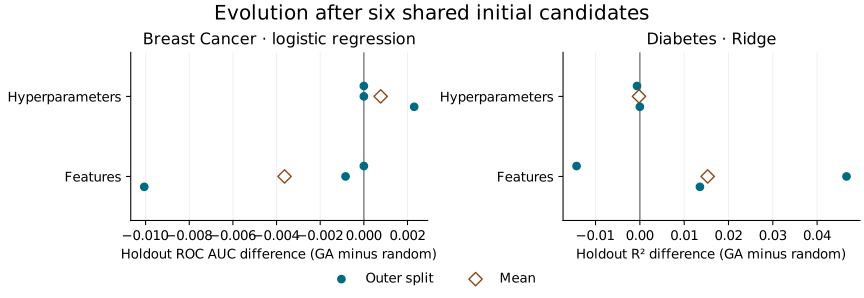
Each value is the mean score on three 25% outer holdouts. Higher is better within each row. On Diabetes, evolution selected masks with higher mean holdout R² even though random continuation scored higher in inner CV. The three outer partitions overlap. This experiment covers two datasets and measures quality per evaluation. Its reproduction script and all twelve pairs are in benchmarks/results/performance-v2/shared-initialization.json in the repository.
How much did another six candidates buy?
With three CV folds, six additional distinct candidates cost 18 more fold fits. On Diabetes, the genetic feature selector improved mean held-out R² from 0.4376 at six candidates to 0.4777 at twelve. Random continuation reached 0.4473 at the same budget. On Breast Cancer, increasing the genetic feature search from six to eighteen candidates lowered mean held-out ROC AUC from 0.9917 to 0.9902.
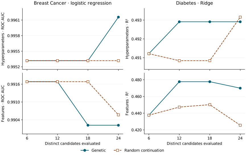
Each point averages the same three outer partitions. Each panel has its own vertical scale. At each budget, inner CV chose the winner before the holdout was scored. In 11 of the 12 genetic runs the winner stayed the same between budgets 12 and 18. Four of those runs later found a higher inner CV score. The holdout score ultimately rose in two of the eleven runs, fell in two and tied in seven. A single flat interval gave little guidance on when to stop.
Download the per-split candidates, CV scores and holdout scores (JSON).
Should a small initial population try a different kernel in every slot?
In this SVM experiment, forcing a third distinct kernel changed mean held-out balanced accuracy by at most 0.18 percentage points per dataset. A repeated kernel can still be worth evaluating when another hyperparameter changes.
Each GASearchCV run started with three candidates, including the estimator default (rbf, C=1). The search sampled from four equally weighted kernels and a log-uniform range for C. In 24 of 64 runs, another candidate used rbf at a different C. For each such run, we replaced that kernel with each unused kernel in turn, keeping its C and the other two candidates fixed. Each alternative had the same nine fold fits. Three-fold CV selected its winner before we scored it on the outer holdout.
Choosing an unused kernel uniformly improved the expected holdout score in eight of those 24 runs, reduced it in two and tied in fourteen. The expectation averages the two possible replacements. The study used Iris, Wine, Breast Cancer and a 450-observation Digits subset, with two outer splits and eight search seeds per dataset. It covers the initial population only.
To check coverage in your own run, inspect cv_results_["params"]: two entries with the same kernel and different C values represent distinct model fits. See the categorical sampling rules or download all candidates, splits and scores (JSON).
Does resuming a checkpoint change search quality at the same budget?
At 24 distinct candidates, resumed and uninterrupted searches tied on held-out score in 10 of 12 comparisons. At 36 candidates, feature selection on Wine improved on one split and tied on two. On Diabetes it scored lower on two splits and tied on one.
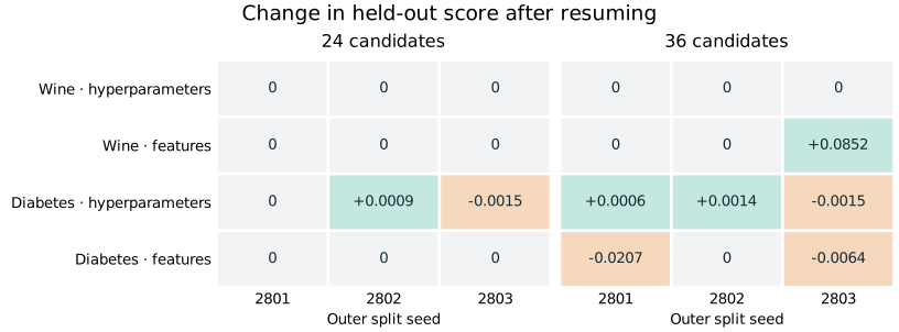
Each cell subtracts the uninterrupted winner's score from the resumed winner's score on the same 25% outer holdout. Positive values favor resuming. Wine used a decision tree and balanced accuracy. Diabetes used Ridge and R². The three outer splits within each dataset overlap.
Both methods started with the same 17 or 18 candidates and their CV scores. At budgets of 24 and 36, each method used 72 and 108 inner fold fits respectively to rank the candidates in its prefix. Only then was the winner refitted and scored on the holdout. These budgets compare solution quality per evaluation. They do not measure elapsed time.
Download per-split winners, scores and the reproduction script (JSON). To resume your own search, see Resume from a checkpoint.
Why Bayesmark?
Frameworks like Optuna do not benchmark on ad-hoc problems. The Optuna team uses tools such as kurobako and benchmark suites such as Bayesmark (originally from the NeurIPS 2020 Black-Box Optimization Challenge). Bayesmark's recipe is deliberately simple and framework-agnostic:
- A handful of small, standard scikit-learn datasets.
- A handful of standard scikit-learn estimators, each with a fixed search space.
- Every optimizer receives a candidate budget. The harness records actual evaluation counts.
- Each task is repeated over several seeds, and the best cross-validation score is reported.
Because the datasets and search spaces are fixed and public, any optimizer — Optuna, random search, or a genetic algorithm — can be dropped into the same harness and compared fairly. That is exactly what the benchmark script in this repository does.
Faithful reproduction
The per-model search spaces below are copied verbatim from Bayesmark's API_CONFIG. The only adaptation: Bayesmark searches some bounded parameters in logit space, a warp that none of the three optimizers expose directly, so those parameters are searched on their natural bounded range for every optimizer. This keeps the comparison even.
What We Compare
| Optimizer | Library | Strategy |
|---|---|---|
GASearchCV | sklearn-genetic-opt | Evolutionary search (DEAP) with smart initialization |
| Optuna | optuna | Bayesian optimization with the TPE sampler |
RandomizedSearchCV | scikit-learn | Random sampling — the standard strong baseline |
Datasets
From Bayesmark's DATA_LOADERS (we drop boston, which modern scikit-learn removed):
| Dataset | Task | Loader |
|---|---|---|
| iris | classification | load_iris |
| wine | classification | load_wine |
| breast | classification | load_breast_cancer |
| digits | classification | load_digits |
| diabetes | regression | load_diabetes |
Classification is scored by accuracy; regression by mean squared error (optimized as neg_mean_squared_error).
Models and Search Spaces
Copied from Bayesmark's API_CONFIG. log parameters use a log-uniform distribution; linear/logit parameters use a uniform distribution on the listed range.
| Model | Parameter | Type | Scale | Range |
|---|---|---|---|---|
| knn | n_neighbors | int | linear | 1 – 25 |
p | int | linear | 1 – 4 | |
| svm | C | real | log | 1.0 – 1e3 |
gamma | real | log | 1e-4 – 1e-3 | |
tol | real | log | 1e-5 – 1e-1 | |
| dt | max_depth | int | linear | 1 – 15 |
min_samples_split | real | logit | 0.01 – 0.99 | |
min_samples_leaf | real | logit | 0.01 – 0.49 | |
min_weight_fraction_leaf | real | logit | 0.01 – 0.49 | |
max_features | real | logit | 0.01 – 0.99 | |
min_impurity_decrease | real | linear | 0.0 – 0.5 | |
| rf | (same six as dt) | |||
| ada | n_estimators | int | linear | 10 – 100 |
learning_rate | real | log | 1e-4 – 1e1 | |
| lasso / linear | C (clf) / alpha (reg) | real | log | 1e-2 – 1e2 |
intercept_scaling (clf) | real | log | 1e-2 – 1e2 |
Scaled models (knn, svm, mlp, lasso, linear) are wrapped in a StandardScaler pipeline.
Equal Budget, Fair Comparison
The current Bayesmark runner gives each method the same ceiling. Randomized search requests one candidate per iteration, and Optuna requests one candidate per trial. The GA starts with up to eight candidates and proposes up to two offspring per population member per generation. It takes only whole generations within the budget, disables local refinement and caches repeated configurations.
For example, with --budget 48, a population of eight fits two full generations, for at most 40 candidate evaluations (8 + 16 + 16). With three folds, 40 evaluations require 120 fold fits. Randomized search can use all 48 evaluations, or 144 fold fits. Inspect mean_evaluations, mean_seconds and the number of successful seeds (n_seeds) in the Bayesmark JSON report.
The separate benchmarks/benchmark_fit.py harness also supports finalist validation. Its actual_cross_validate_calls_mean counts candidate evaluations across search and finalist validation. Its cv_fold_fits_mean counts the underlying fold fits. Wall time includes the final full-data refit. A candidate evaluated on one fold and promoted to three folds therefore contributes four fold fits in this workflow.
Running It Yourself
From a repository checkout, install the benchmark extra to include Optuna in the comparison:
python -m pip install -e ".[benchmark]"Then run the script from the repository root:
# Fast smoke run (a few datasets/models, small budget)
python benchmarks/benchmark_bayesmark.py --quick

# Full reproducible run with a JSON report
python benchmarks/benchmark_bayesmark.py \
    --datasets iris wine breast diabetes \
    --models knn svm dt rf ada \
    --optimizers gasearch optuna randomized \
    --budget 64 --seeds 3 \
    --output-json benchmarks/bayesmark.json

# Pick a single task to inspect closely
python benchmarks/benchmark_bayesmark.py --datasets wine --models svm --budget 80
If Optuna is not installed, the script prints a note and simply runs the remaining optimizers.
Results
The table below reports the mean ± standard deviation of the best cross-validation score across seeds. For classification the metric is accuracy (higher is better); for regression it is MSE (lower is better). The winner column marks the optimizer with the best mean on the optimized objective.
These historical results used a nominal budget of 48, three seeds and three-fold CV. The current runner uses the whole-generation cap described above. Use its JSON report for the realized counts of a new run.
| dataset | model | metric | gasearch | optuna | randomized | winner |
|---|---|---|---|---|---|---|
| wine | knn | accuracy ↑ | 0.9832 ± 0.0046 | 0.9832 ± 0.0046 | 0.9813 ± 0.0027 | gasearch |
| wine | svm | accuracy ↑ | 0.9869 ± 0.0053 | 0.9851 ± 0.0026 | 0.9850 ± 0.0027 | gasearch |
| wine | dt | accuracy ↑ | 0.8520 ± 0.0117 | 0.8651 ± 0.0091 | 0.8463 ± 0.0312 | optuna |
| wine | rf | accuracy ↑ | 0.9645 ± 0.0095 | 0.9719 ± 0.0000 | 0.9532 ± 0.0096 | optuna |
| breast | knn | accuracy ↑ | 0.9684 ± 0.0014 | 0.9695 ± 0.0008 | 0.9678 ± 0.0008 | optuna |
| breast | svm | accuracy ↑ | 0.9789 ± 0.0000 | 0.9783 ± 0.0008 | 0.9783 ± 0.0008 | gasearch |
| breast | dt | accuracy ↑ | 0.9133 ± 0.0030 | 0.9151 ± 0.0017 | 0.9133 ± 0.0030 | optuna |
| breast | rf | accuracy ↑ | 0.9256 ± 0.0054 | 0.9285 ± 0.0072 | 0.9215 ± 0.0060 | optuna |
| diabetes | knn | MSE ↓ | 3223.40 ± 114.3 | 3229.59 ± 107.3 | 3223.47 ± 114.4 | gasearch |
| diabetes | svm | MSE ↓ | 3035.66 ± 28.6 | 3034.17 ± 30.1 | 3053.55 ± 33.9 | optuna |
| diabetes | dt | MSE ↓ | 3994.28 ± 183.6 | 3837.88 ± 106.5 | 3852.95 ± 159.9 | optuna |
| diabetes | rf | MSE ↓ | 3553.56 ± 219.1 | 3320.70 ± 52.5 | 3498.15 ± 188.9 | optuna |
↑ higher is better, ↓ lower is better. Bold marks the best mean per row.
Across these twelve rows, the GA had higher mean inner CV scores than randomized search on ten tasks. Optuna had the best mean on each tree and forest task. Small score differences on the folds used for tuning warrant a separate holdout check.
Does more budget close the gap?
These historical runs compare nominal budgets of 48 and 96 on four tasks.
| task | metric | gasearch 48 → 96 | optuna 48 → 96 | verdict change |
|---|---|---|---|---|
| wine / dt | accuracy ↑ | 0.8520 → 0.8690 | 0.8651 → 0.8670 | optuna → gasearch wins |
| diabetes / rf | MSE ↓ | 3553.6 → 3295.8 | 3320.7 → 3259.6 | gap 233 → 36 |
| breast / rf | accuracy ↑ | 0.9256 → 0.9303 | 0.9285 → 0.9391 | still optuna |
| wine / rf | accuracy ↑ | 0.9645 → 0.9664 | 0.9719 → 0.9776 | still optuna |
The larger budget reversed the ordering on Wine/tree and narrowed the gap on Diabetes/forest. Optuna retained the higher mean accuracy on both random-forest classification tasks.
Mixed and Conditional Spaces
Bayesmark's spaces are almost entirely numeric — the home turf of Bayesian optimizers. Real hyperparameter tuning is often mixed and conditional: categorical switches that turn whole regions of the space on or off. The --suite mixed benchmark builds exactly that kind of space, where sklearn-genetic-opt's native categorical handling and population-based crossover have more to work with.
python benchmarks/benchmark_bayesmark.py --suite mixed --budget 96 --seeds 3Two estimators, both with categorical and conditionally-relevant parameters:
| Model | Categorical / conditional parameters |
|---|---|
svc_mixed (SVC) | kernel ∈ {linear, rbf, poly, sigmoid} (makes degree/coef0/gamma relevant only for some kernels), class_weight, shrinking |
histgb_mixed (HistGradientBoosting) | max_depth ∈ {None, 3, 5, 7, 9} (unbounded vs capped), interaction_cst ∈ {None, "no_interactions"}, plus numeric leaf/learning-rate parameters |
Run with budget = 64, 3 seeds, 3-fold CV (diabetes/svc_mixed is skipped — SVC is a classifier here):
| dataset | model | metric | gasearch | optuna | randomized | winner |
|---|---|---|---|---|---|---|
| wine | svc_mixed | accuracy ↑ | 0.9851 ± 0.0026 | 0.9868 ± 0.0053 | 0.9868 ± 0.0053 | optuna |
| wine | histgb_mixed | accuracy ↑ | 0.9831 ± 0.0080 | 0.9832 ± 0.0046 | 0.9794 ± 0.0054 | optuna |
| breast | svc_mixed | accuracy ↑ | 0.9801 ± 0.0022 | 0.9801 ± 0.0017 | 0.9783 ± 0.0008 | tie |
| breast | histgb_mixed | accuracy ↑ | 0.9713 ± 0.0054 | 0.9719 ± 0.0014 | 0.9707 ± 0.0051 | optuna |
| diabetes | histgb_mixed | MSE ↓ | 3248.9 ± 10.6 | 3212.7 ± 13.1 | 3231.2 ± 18.6 | optuna |
Optuna matched or exceeded the GA mean in all five rows. The CASH experiment below tests a different decision: choosing the estimator family together with its hyperparameters.
CASH: Algorithm Selection + Tuning
In a CASH (Combined Algorithm Selection and Hyperparameter optimization) problem the optimizer must choose which estimator family to use and tune that family's hyperparameters at the same time. The space is deeply conditional: svm_gamma only matters when the SVM is selected, rf_max_depth only for the random forest, and so on.
The benchmark (benchmarks/benchmark_cash.py) searches across five families — RBF SVM, random forest, histogram gradient boosting, logistic regression, and k-NN — a 15-dimensional conditional space:
python benchmarks/benchmark_cash.py --dataset synth --budget 100 --seeds 3It is deliberately a fair fight:
- Optuna uses its native, define-by-run conditional API — it suggests the family first, then only that family's parameters. Conditional spaces are a headline Optuna strength, so it is not handicapped.
GASearchCVandRandomizedSearchCVget the same problem through a flatCASHClassifiermeta-estimator that exposes every family's parameters and routes to the selected one atfit. Both carry the flat-encoding tax of inactive genes.
The dataset has real headroom — a 1500×25 make_classification with a non-linear, multi-cluster boundary that tops out around 0.86 (it does not saturate near 1.0), so the estimator family genuinely matters and there is room to separate.
The historical run below used 184 realized candidate evaluations per optimizer, three seeds and three-fold CV. The current CASH runner disables local refinement and gives each baseline the number of CV evaluations actually used by the GA on that seed.
| optimizer | mean accuracy ± std | best | mean evals | mean wall time |
|---|---|---|---|---|
| optuna | 0.8636 ± 0.0050 | 0.8707 | 184 | 59 s |
| randomized | 0.8591 ± 0.0055 | 0.8667 | 184 | 27 s |
| gasearch | 0.8582 ± 0.0087 | 0.8693 | 184 | 205 s |
In this run, Optuna had the highest mean CV accuracy and randomized search had the shortest mean runtime. One difference between methods is how they encode the family choice. Optuna proposes parameters for the active family. The flat GA encoding also carries parameters for inactive families. The benchmark compares the complete methods and does not isolate the effect of that encoding.
How to Interpret a Benchmark
- For compute efficiency, compare realized fold fits and elapsed time on the same hardware. Different candidates can have very different training costs.
- For solution quality, choose candidates using inner CV and evaluate winners on untouched outer data. Report the metric and the per-split differences.
- To evaluate a new search policy, reserve whole datasets before choosing defaults. Additional seeds on familiar tasks measure split variability while leaving the choice of tasks fixed.
See Also
- Comparing Search Methods — a single-task, copy-pasteable comparison with full code.
- Advanced Optimizer Control — diversity control, local search and fitness sharing.
- When to Use — picking the right search method for your problem.
- Bayesmark and kurobako — the upstream benchmark tooling.