Development version

This is the latest (dev) documentation. It may contain unreleased features or breaking changes. For the stable release, use stable.

Estimated reading time: 15 minutes
Difficulty: Beginner
Prerequisites: Python, pip, basic sklearn knowledge (train_test_split, classifiers)

Getting Started with GASearchCV: Hyperparameter Tuning and Feature Selection

This page walks through the two workflows you will use most:

• Hyperparameter tuning with GASearchCV
• Feature selection with GAFeatureSelectionCV

Every code block below is executed to build this page, so what you copy is exactly what ran — including the outputs and figures.

Prerequisites

• sklearn-genetic-opt installed (pip install sklearn-genetic-opt)
• Optional plotting extra for the figures: pip install sklearn-genetic-opt[plot]
• Basic familiarity with scikit-learn's fit / predict API

Hyperparameter Tuning

We tune an MLPClassifier on the handwritten digits dataset (10 classes, 64 pixel features). First, the imports and data:

import numpy as np
from sklearn.datasets import load_digits
from sklearn.metrics import accuracy_score
from sklearn.model_selection import StratifiedKFold, train_test_split
from sklearn.neural_network import MLPClassifier

from sklearn_genetic import EvolutionConfig, GASearchCV, PopulationConfig, RuntimeConfig
from sklearn_genetic.space import Categorical, Continuous, Integer

RANDOM_STATE = 42

X, y = load_digits(return_X_y=True)
X_train, X_test, y_train, y_test = train_test_split(
    X, y, test_size=0.33, stratify=y, random_state=RANDOM_STATE
)
cv = StratifiedKFold(n_splits=3, shuffle=True, random_state=RANDOM_STATE)
print(f"train={X_train.shape}  test={X_test.shape}  classes={len(np.unique(y))}")

train=(1203, 64)  test=(594, 64)  classes=10

Define the search space

The keys in param_grid are estimator parameter names. Each value is a space the genetic algorithm samples from:

• Integer — whole numbers in a range
• Continuous — floats in a range (optionally distribution="log-uniform")
• Categorical — a fixed list of choices

param_grid = {
    "hidden_layer_sizes": Categorical([(32,), (64,), (32, 16)]),
    "alpha": Continuous(1e-5, 1e-1, distribution="log-uniform"),
    "learning_rate_init": Continuous(1e-4, 1e-1, distribution="log-uniform"),
    "activation": Categorical(["relu", "tanh"]),
    "batch_size": Integer(32, 256),
}

Configure and run the search

GASearchCV is configured with small config objects. EvolutionConfig controls the population and generations; PopulationConfig(initializer="smart") builds a diverse, well-spread starting population; RuntimeConfig controls parallelism and logging.

clf = MLPClassifier(max_iter=150, early_stopping=True, random_state=RANDOM_STATE)

search = GASearchCV(
    estimator=clf,
    random_state=RANDOM_STATE,
    cv=cv,
    scoring="accuracy",
    param_grid=param_grid,
    evolution_config=EvolutionConfig(population_size=8, generations=6),
    population_config=PopulationConfig(initializer="smart"),
    runtime_config=RuntimeConfig(n_jobs=-1, verbose=False),
)

search.fit(X_train, y_train)

print(f"Best CV accuracy : {search.best_score_:.4f}")
print(f"Best parameters  : {search.best_params_}")

Best CV accuracy : 0.9584
Best parameters  : {'hidden_layer_sizes': (64,), 'alpha': 0.00027470715996250945, 'learning_rate_init': 0.003590489008293675, 'activation': 'relu', 'batch_size': 70}

After fitting, GASearchCV behaves like any fitted scikit-learn estimator — it has already refit the best configuration on all of X_train:

y_pred = search.predict(X_test)
print(f"Holdout accuracy : {accuracy_score(y_test, y_pred):.4f}")

Holdout accuracy : 0.9579

Reading the evolution

Each generation is logged. Inspect the full history as a DataFrame — the columns explain how the population improved and how diverse it stayed:

Column	Meaning
gen	generation number
fitness	mean CV score in the generation
fitness_best	best CV score found so far
genotype_diversity	1.0 = diverse, 0.0 = converged
unique_individual_ratio	fraction of distinct configurations
stagnation_generations	consecutive generations without improvement

import pandas as pd

history = pd.DataFrame(search.history)
print(history[["gen", "fitness", "fitness_best", "genotype_diversity",
               "unique_individual_ratio", "stagnation_generations"]].to_string(index=False))

 gen  fitness  fitness_best  genotype_diversity  unique_individual_ratio  stagnation_generations
   0 0.753325      0.946800            0.685714                    1.000                       0
   1 0.932253      0.946800            0.485714                    0.875                       1
   2 0.943890      0.955112            0.314286                    0.750                       0
   3 0.945449      0.955112            0.371429                    0.750                       1
   4 0.948462      0.955112            0.314286                    0.750                       2
   5 0.951995      0.955112            0.314286                    0.750                       3
   6 0.953242      0.958437            0.228571                    0.625                       0

fit_stats_ summarizes what the search actually spent — useful for spotting wasted effort (e.g. many skipped_invalid_candidates):

for key, value in search.fit_stats_.items():
    print(f"{key}: {value}")

evaluated_candidates: 104
unique_candidates: 102
cross_validate_calls: 102
cache_hits: 2
duplicate_candidates: 0
skipped_invalid_candidates: 0
population_parallel_batches: 7
population_serial_batches: 0
random_immigrants: 0
local_refinement_candidates: 0

Visualize convergence

With the [plot] extra installed, plot_fitness_evolution shows the best score climbing over generations, and plot_search_overview gives a compact diagnostic dashboard.

import matplotlib.pyplot as plt
from sklearn_genetic.plots import plot_search_overview

plot_search_overview(search, top_k=6)
plt.tight_layout()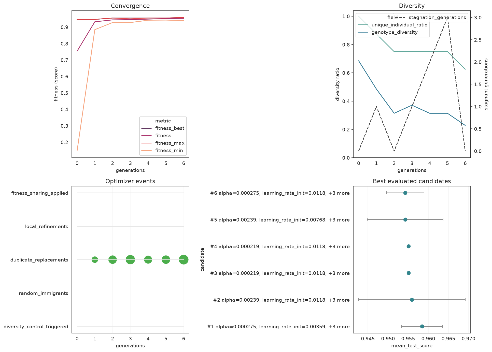

from sklearn_genetic.plots import plot_parameter_evolution

plot_parameter_evolution(search, parameters=["alpha", "learning_rate_init", "batch_size"])
plt.tight_layout()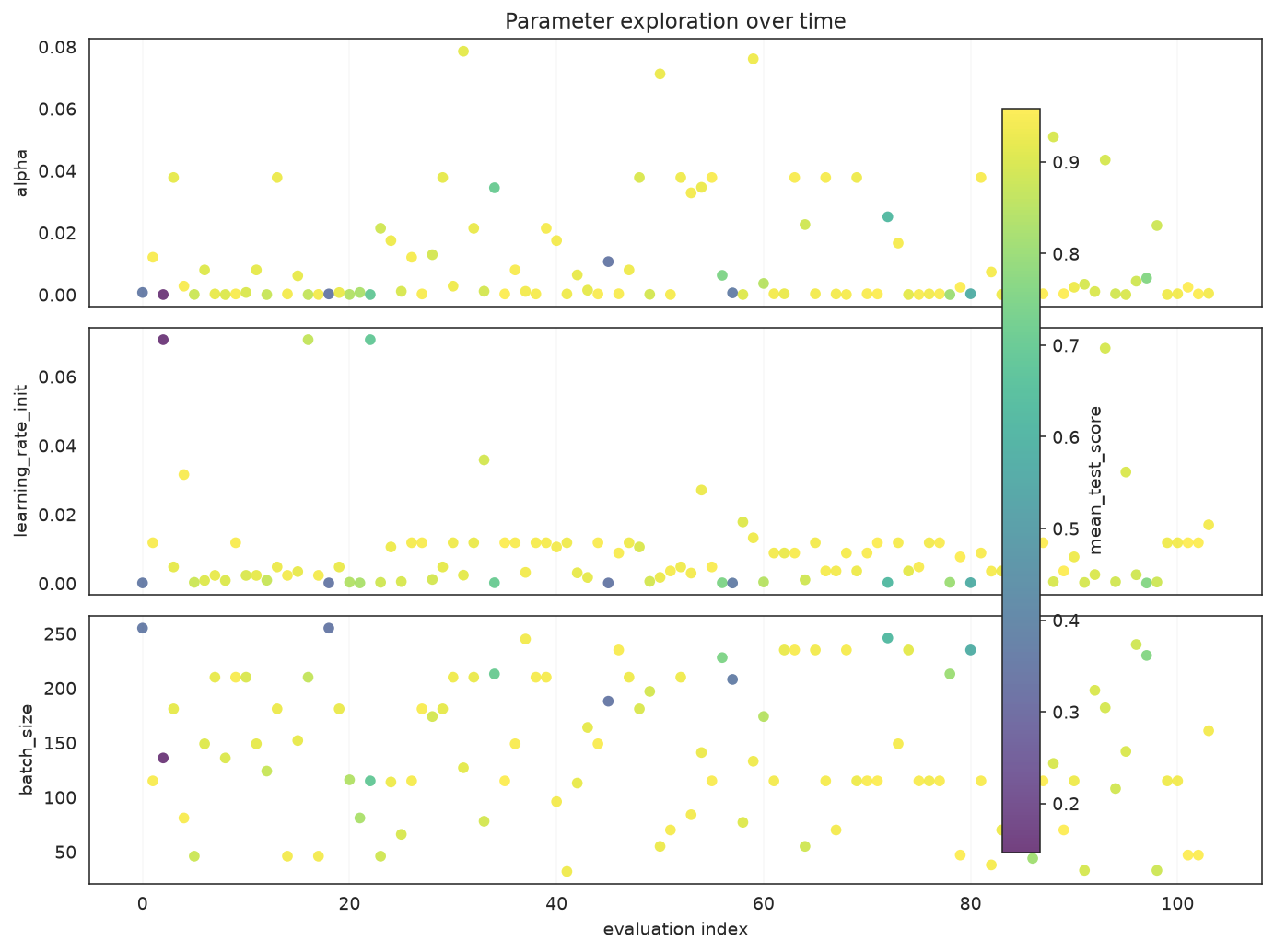

Feature Selection

GAFeatureSelectionCV searches for the most useful subset of columns. To make the task concrete we take the Iris dataset and bolt on 10 columns of pure noise; a good selector should keep the real measurements and discard the noise.

from sklearn.datasets import load_iris
from sklearn.svm import SVC

from sklearn_genetic import GAFeatureSelectionCV

iris = load_iris()
rng = np.random.default_rng(RANDOM_STATE)
noise = rng.uniform(0, 10, size=(iris.data.shape[0], 10))
X_fs = np.hstack([iris.data, noise])
feature_names = list(iris.feature_names) + [f"noise_{i}" for i in range(10)]
y_fs = iris.target

Xtr, Xte, ytr, yte = train_test_split(
    X_fs, y_fs, test_size=0.33, stratify=y_fs, random_state=RANDOM_STATE
)

selector = GAFeatureSelectionCV(
    estimator=SVC(gamma="auto"),
    random_state=RANDOM_STATE,
    cv=3,
    scoring="accuracy",
    evolution_config=EvolutionConfig(population_size=10, generations=8,
                                     elitism=True, keep_top_k=2),
    population_config=PopulationConfig(initializer="smart"),
    runtime_config=RuntimeConfig(n_jobs=-1, verbose=False),
)
selector.fit(Xtr, ytr)

selected = [name for name, keep in zip(feature_names, selector.support_) if keep]
print(f"Selected {len(selected)} of {len(feature_names)} features:")
for name in selected:
    print(f"  - {name}")
print(f"Holdout accuracy : {accuracy_score(yte, selector.predict(Xte)):.4f}")

Selected 3 of 14 features:
  - sepal length (cm)
  - sepal width (cm)
  - petal length (cm)
Holdout accuracy : 0.9800

support_ is a boolean mask (True = kept). The search keeps the informative Iris measurements and drops most of the noise columns. Visualize the mask:

from sklearn_genetic.plots import plot_feature_selection

plot_feature_selection(selector, feature_names=feature_names)
plt.tight_layout()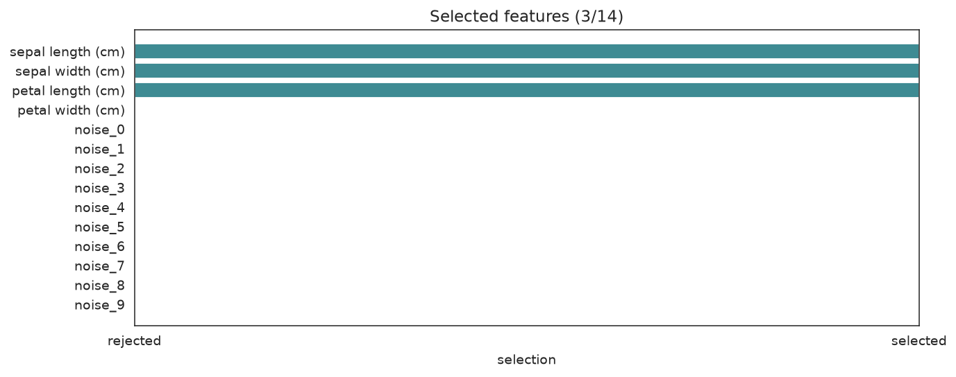

Tips & Gotchas

• Set RuntimeConfig(verbose=True) to watch the per-generation log live.
• PopulationConfig(initializer="smart") is strongly recommended — it usually finds better solutions faster than a purely random start.
• If accuracy is already near 1.0 on your data, switch to a more discriminative metric (e.g. roc_auc, balanced_accuracy).
• Check fit_stats_["skipped_invalid_candidates"] after fitting — a non-zero value means some sampled configurations raised errors during fit.

See Also

• How Hyperparameter Optimization Works — understand the theory behind different search methods
• Choosing the Right Search Space — pick optimal parameter bounds
• Common Hyperparameter Tuning Mistakes — avoid the most frequent pitfalls
• Cross-Validation in Hyperparameter Search — understand generation logs and convergence
• Random Forest Hyperparameter Tuning — first real tutorial
• Troubleshooting — if something doesn't work