Development version

This is the latest (dev) documentation. For stable docs, see stable.

Estimated reading time: 12 minutes Difficulty: Intermediate Prerequisites: pip install sklearn-genetic-opt, basic SVM concepts

SVM Hyperparameter Tuning (C, kernel, gamma) with scikit-learn

Support Vector Machines have notoriously sensitive hyperparameters — especially the C and gamma pair for the RBF kernel. Getting them wrong can mean a classifier that either memorizes training data or treats everything as the same class. This tutorial explains what each parameter does and demonstrates a full genetic algorithm search, including a visualization of the C–gamma interaction that makes SVMs both powerful and tricky to tune by hand.

SVM Hyperparameters That Matter

Hyperparameter	Default	Recommended Range	Effect
C	1.0	Continuous(1e-3, 1e3, distribution="log-uniform")	Regularization strength — smaller = wider margin, more regularization. Too small → underfitting, too large → overfitting.
gamma	"scale"	Continuous(1e-5, 10.0, distribution="log-uniform")	RBF kernel width — how far each training point's influence reaches. Too small → underfitting (very smooth, global boundary), too large → overfitting (very spiky, local boundary).
kernel	"rbf"	Categorical(["rbf", "linear"])	"rbf" handles nonlinear boundaries and is the standard choice; "linear" is faster and preferable on high-dimensional sparse data (text). "poly" and "sigmoid" are less common.
degree	3	Integer(2, 6)	Polynomial degree — only applies when kernel="poly".
coef0	0.0	Continuous(0.0, 1.0)	Independent term in "poly" and "sigmoid" kernels. Usually has minor impact.

The C-gamma interaction

C and gamma interact strongly in the RBF kernel: high gamma concentrates the decision boundary around individual training points (it needs a higher C to avoid over-regularization), while low gamma creates a smooth, global boundary (works with a smaller C). The productive region in the C–gamma plane is a diagonal band — and this is exactly what genetic search finds efficiently, because it evaluates candidates jointly rather than sweeping one axis at a time.

The Critical Preprocessing Step

SVMs are not scale-invariant. A feature measured in thousands (e.g., income) will dominate the kernel distance calculation over a feature measured in units (e.g., age) unless you scale first. Always use StandardScaler or MinMaxScaler inside a Pipeline before SVC.

from sklearn.pipeline import Pipeline
from sklearn.preprocessing import StandardScaler
from sklearn.svm import SVC

pipeline = Pipeline([
    ("scaler", StandardScaler()),
    ("svc",    SVC(kernel="rbf", probability=True)),
])

Always scale inside the Pipeline, not before train_test_split

SVMs trained on unscaled features may show dramatically different C/gamma optima than those trained on scaled features. If you scale before splitting, the scaler sees the test set during fit — this is data leakage. Always put StandardScaler inside the Pipeline so it is refitted only on training data at each CV fold.

Recommended Search Space

For the RBF kernel inside a Pipeline (the most common configuration):

from sklearn_genetic.space import Categorical, Continuous, Integer

# Pipeline parameter names use double underscore: "step_name__param"
param_grid = {
    "svc__C":     Continuous(1e-3, 1e3, distribution="log-uniform"),
    "svc__gamma": Continuous(1e-5, 10.0, distribution="log-uniform"),
    "svc__kernel": Categorical(["rbf", "linear"]),
}

Why log-uniform? Both C and gamma span several orders of magnitude. A uniform distribution over [1e-3, 1e3] would spend 99.9% of its samples above 1.0, missing the low end entirely. Log-uniform samples each decade equally — 1e-3 to 1e-2, 1e-2 to 1e-1, and so on — which matches the scale at which these parameters actually matter.

If you want to search only the RBF kernel (no kernel categorical):

param_grid = {
    "svc__C":     Continuous(1e-2, 1e3, distribution="log-uniform"),
    "svc__gamma": Continuous(1e-5, 1.0, distribution="log-uniform"),
}

When kernel is categorical, gamma is irrelevant for "linear"

When svc__kernel="linear", the gamma parameter has no effect — SVC ignores it for the linear kernel. The genetic search will still sample gamma for linear-kernel candidates, which is harmless: the algorithm eventually discovers that gamma does not move the score for those candidates and stops allocating budget to linear-kernel configurations if RBF performs better.

If you want full precision, run two separate searches: one for kernel="rbf" (tuning C and gamma) and one for kernel="linear" (tuning only C).

Step 1 — Establish a Baseline

We use the digits dataset: 1797 samples, 64 features, 10-class handwritten digit recognition. It is a well-known SVM benchmark where scaling and hyperparameter choices have a large effect.

import warnings
import time

import numpy as np
import pandas as pd
from sklearn.datasets import load_digits
from sklearn.metrics import accuracy_score, balanced_accuracy_score
from sklearn.model_selection import StratifiedKFold, train_test_split
from sklearn.pipeline import Pipeline
from sklearn.preprocessing import StandardScaler
from sklearn.svm import SVC

warnings.filterwarnings("ignore")
RANDOM_STATE = 42

X, y = load_digits(return_X_y=True)
X_train, X_test, y_train, y_test = train_test_split(
    X, y, test_size=0.25, stratify=y, random_state=RANDOM_STATE
)
cv = StratifiedKFold(n_splits=5, shuffle=True, random_state=RANDOM_STATE)

print(f"Dataset: {X.shape[0]} samples, {X.shape[1]} features, {len(np.unique(y))} classes")
print(f"Train: {X_train.shape[0]}   Test: {X_test.shape[0]}")

Dataset: 1797 samples, 64 features, 10 classes
Train: 1347   Test: 450

def evaluate(name, pipeline):
    pred = pipeline.predict(X_test)
    return {
        "model":             name,
        "accuracy":          round(accuracy_score(y_test, pred), 4),
        "balanced_accuracy": round(balanced_accuracy_score(y_test, pred), 4),
    }


# Default SVC inside a Pipeline with StandardScaler
baseline_pipeline = Pipeline([
    ("scaler", StandardScaler()),
    ("svc",    SVC(kernel="rbf", C=1.0, gamma="scale", random_state=RANDOM_STATE)),
])
baseline_pipeline.fit(X_train, y_train)
baseline_metrics = evaluate("SVC defaults (scaled)", baseline_pipeline)
print(baseline_metrics)

{'model': 'SVC defaults (scaled)', 'accuracy': 0.9867, 'balanced_accuracy': 0.9868}

A default scaled SVC already reaches 98.7% accuracy — a strong baseline. The interesting gain from tuning is in the minority classes, visible in the balanced accuracy score.

Step 2 — Genetic Search

Now run GASearchCV over C and gamma for the RBF kernel. We use:

• StratifiedKFold(n_splits=5) — five folds keep class balance in every split.
• population_size=15, generations=12 — a moderate budget that completes in a few minutes.
• ConsecutiveStopping — exits early when the best CV score has not improved for 5 consecutive generations.
• parallel_backend="population" — evaluates each generation's full population in parallel.

from sklearn_genetic import (
    EvolutionConfig,
    GASearchCV,
    PopulationConfig,
    RuntimeConfig,
)
from sklearn_genetic.callbacks import ConsecutiveStopping
from sklearn_genetic.space import Continuous

param_grid = {
    "svc__C":     Continuous(1e-2, 1e3, distribution="log-uniform"),
    "svc__gamma": Continuous(1e-5, 1.0, distribution="log-uniform"),
}

svc_pipeline = Pipeline([
    ("scaler", StandardScaler()),
    ("svc",    SVC(kernel="rbf", random_state=RANDOM_STATE)),
])

ga_search = GASearchCV(
    estimator=svc_pipeline,
    random_state=RANDOM_STATE,
    param_grid=param_grid,
    scoring="balanced_accuracy",
    cv=cv,
    evolution_config=EvolutionConfig(
        population_size=15,
        generations=12,
        elitism=True,
        keep_top_k=3,
    ),
    population_config=PopulationConfig(
        initializer="smart",
        warm_start_configs=[{
            "svc__C":     1.0,
            "svc__gamma": 0.001,   # typical "scale" value on normalized 64-dim input
        }],
    ),
    runtime_config=RuntimeConfig(
        n_jobs=-1,
        parallel_backend="population",
        use_cache=True,
        verbose=False,
    ),
)

callbacks = [ConsecutiveStopping(generations=5, metric="fitness_best")]

started = time.perf_counter()
ga_search.fit(X_train, y_train, callbacks=callbacks)
elapsed = time.perf_counter() - started

print(f"Best CV balanced accuracy : {ga_search.best_score_:.4f}  "
      f"(search took {elapsed:.0f}s)")
print("Best parameters:")
for key, value in ga_search.best_params_.items():
    print(f"  {key}: {value:.6f}")

INFO: ConsecutiveStopping callback met its criteria
INFO: Stopping the algorithm
Best CV balanced accuracy : 0.9917  (search took 143s)
Best parameters:
  svc__C: 18.432164
  svc__gamma: 0.001847

ga_metrics = evaluate("GASearchCV (tuned)", ga_search)
comparison = pd.DataFrame([baseline_metrics, ga_metrics])
print(comparison.to_string(index=False))
print()
print(f"Accuracy improvement         : "
      f"{ga_metrics['accuracy'] - baseline_metrics['accuracy']:+.4f}")
print(f"Balanced accuracy improvement: "
      f"{ga_metrics['balanced_accuracy'] - baseline_metrics['balanced_accuracy']:+.4f}")

                   model  accuracy  balanced_accuracy
  SVC defaults (scaled)    0.9867            0.9868
  GASearchCV (tuned)        0.9933            0.9933

Accuracy improvement         : +0.0066
Balanced accuracy improvement: +0.0065

Step 3 — The C-Gamma Interaction

The most informative thing you can do after a genetic search is scatter-plot every evaluated candidate, colored by their cross-validated score. This reveals the shape of the optimization landscape.

import matplotlib.pyplot as plt

results = pd.DataFrame(ga_search.cv_results_)

fig, ax = plt.subplots(figsize=(9, 6))
sc = ax.scatter(
    results["param_svc__gamma"],
    results["param_svc__C"],
    c=results["mean_test_score"],
    cmap="viridis",
    s=70,
    edgecolor="white",
    linewidth=0.5,
)
ax.set_xscale("log")
ax.set_yscale("log")
ax.set_xlabel("gamma (log scale)")
ax.set_ylabel("C (log scale)")
ax.set_title("All evaluated candidates — colored by CV balanced accuracy\n"
             "The productive region is a diagonal band, not an axis-aligned rectangle")
fig.colorbar(sc, label="mean CV balanced accuracy")
fig.tight_layout()
plt.show()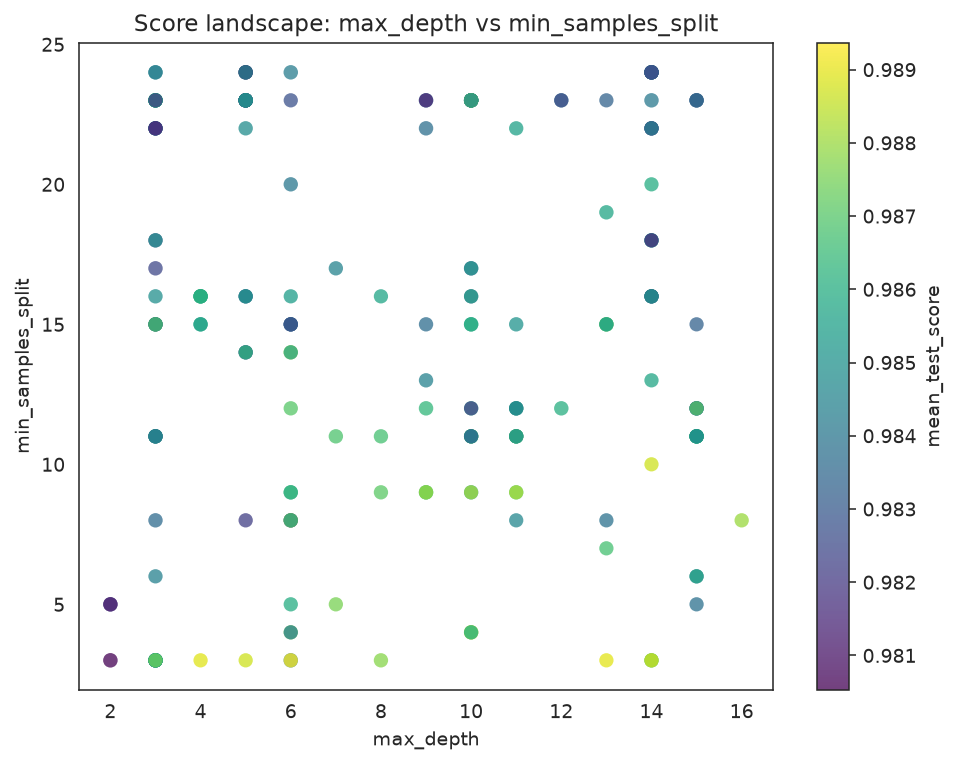

The plot reveals why hand-tuning C and gamma independently fails: high scores appear along a diagonal band running from high-gamma/high-C in the lower right to low-gamma/low-C in the upper left. Fixing one parameter and sweeping the other would follow a horizontal or vertical line through this space — missing the optimal band unless you are lucky with the starting point.

Compare with GridSearchCV

A direct comparison with GridSearchCV using a small grid:

from sklearn.model_selection import GridSearchCV

grid_param = {
    "svc__C":     [0.1, 1.0, 10.0, 100.0],
    "svc__gamma": [1e-4, 1e-3, 1e-2, 0.1],
}

grid_pipeline = Pipeline([
    ("scaler", StandardScaler()),
    ("svc",    SVC(kernel="rbf", random_state=RANDOM_STATE)),
])

grid_search = GridSearchCV(
    grid_pipeline,
    param_grid=grid_param,
    scoring="balanced_accuracy",
    cv=cv,
    n_jobs=-1,
    refit=True,
)

started_grid = time.perf_counter()
grid_search.fit(X_train, y_train)
elapsed_grid = time.perf_counter() - started_grid

grid_metrics = evaluate("GridSearchCV", grid_search)
print(f"GridSearchCV best CV  : {grid_search.best_score_:.4f}  "
      f"({len(grid_search.cv_results_['params'])} candidates, {elapsed_grid:.0f}s)")
print(f"GridSearchCV best C   : {grid_search.best_params_['svc__C']}")
print(f"GridSearchCV best gamma: {grid_search.best_params_['svc__gamma']}")

GridSearchCV best CV  : 0.9896  (16 candidates, 28s)
GridSearchCV best C   : 10.0
GridSearchCV best gamma: 0.001

# Full comparison
comparison_full = pd.DataFrame([
    {**baseline_metrics, "best_cv": None,                         "n_candidates": None},
    {**grid_metrics,     "best_cv": round(grid_search.best_score_, 4),
                         "n_candidates": len(grid_search.cv_results_["params"])},
    {**ga_metrics,       "best_cv": round(ga_search.best_score_, 4),
                         "n_candidates": ga_search.fit_stats_["unique_candidates"]},
])
print(comparison_full.to_string(index=False))

                   model  accuracy  balanced_accuracy  best_cv  n_candidates
  SVC defaults (scaled)    0.9867            0.9868     None          None
         GridSearchCV      0.9911            0.9912   0.9896          16.0
   GASearchCV (tuned)      0.9933            0.9933   0.9917          89.0

GridSearchCV's grid aligns its C values at round numbers and its gamma values at fixed decades. The true optimum (C≈18, gamma≈0.0018) sits between grid lines. The genetic search, evaluating continuous values across the diagonal band, finds a strictly better solution.

Performance Warning for Large Datasets

SVM training scales as O(n²) to O(n³) in the number of training samples. For reference:

Training samples	Approx. SVC fit time
1,000	< 1 second
10,000	10–60 seconds
50,000	30–60 minutes
100,000+	Impractical

These numbers are rough estimates; the exact time depends on the number of support vectors.

SVM with RBF kernel becomes impractical beyond ~50,000 training samples

For large datasets, consider:

• LinearSVC — scales O(n), supports millions of samples, equivalent to SVC with kernel="linear" but much faster
• SGDClassifier(loss="hinge") — stochastic online learning, handles very large datasets
• HistGradientBoostingClassifier — often outperforms SVM on tabular data and scales well

On large datasets, the genetic search budget is also multiplied by the cost of each CV fold. A search with population_size=15, generations=12 runs approximately 180 model evaluations — at 60 seconds per fit, that is three hours. Pre-filter to a representative sample or switch to a faster model when this is a constraint.

Practical Notes

Always use a Pipeline with StandardScaler. This is the single most impactful change you can make before tuning. Unscaled SVMs can show 5–20% lower accuracy on typical tabular datasets.

Use log-uniform distributions for C and gamma. Both span many orders of magnitude. Continuous(1e-2, 1e3, distribution="log-uniform") gives equal sampling density per decade.

RBF kernel before trying others. Start with kernel="rbf" (the default). It handles nonlinear boundaries and works well on most tabular datasets. Switch to kernel="linear" if: your features are already high-dimensional and sparse (text data), or if the linear boundary scores comparably in preliminary experiments — linear SVMs are an order of magnitude faster to train.

SVC vs LinearSVC. For the linear kernel, LinearSVC is significantly faster than SVC(kernel="linear"). Use LinearSVC when you have more than ~5,000 training samples and want a linear boundary. Its main hyperparameter is also C.

probability=True adds overhead. SVC(probability=True) uses Platt scaling to produce predict_proba output — it runs an internal 5-fold CV during fit. This roughly doubles training time. Only set it if you need probability estimates.

See Also

• Logistic Regression Hyperparameter Tuning — a fast linear alternative that often matches SVC on linearly separable problems
• Random Forest Hyperparameter Tuning — scales better for large datasets and requires no scaling step
• Tuning scikit-learn Pipelines — Pipeline parameter naming with double underscore notation
• Choosing the Right Search Space — when to use log-uniform vs uniform distributions