
Development version
This is the latest (dev) documentation. It may contain unreleased features or breaking changes. For the stable release, use stable.
Estimated reading time: 15 minutes Difficulty: Intermediate Prerequisites: scikit-learn, sklearn-genetic-opt (pip install sklearn-genetic-opt)
Random Forest Hyperparameter Tuning with Genetic Algorithms
Random Forest is one of the most reliable off-the-shelf classifiers, but its performance depends heavily on the right hyperparameter combination. Eight key hyperparameters interact with each other — n_estimators, max_depth, min_samples_split, and more — and tuning them jointly is what separates a good model from a great one. This tutorial shows exactly which parameters to tune, what ranges to use, and walks through a full search with GASearchCV from sklearn-genetic-opt — including a before-and-after comparison and interaction visualization.
Which Hyperparameters Actually Matter?
Random Forest has more knobs than most people realize. Here is every hyperparameter worth considering, along with its default, a recommended search range, and — critically — why it matters.
| Hyperparameter | Default | Recommended Range | Why it matters |
|---|---|---|---|
n_estimators | 100 | Integer(50, 500) | More trees reduce variance but add time. Gains flatten above ~200 on most datasets. |
max_depth | None | Integer(3, 25) | Fully-grown trees (None) memorize training data. Capping depth is the primary regularization lever. |
min_samples_split | 2 | Integer(2, 20) | Requires at least N samples to attempt a split. Higher values smooth decision boundaries and resist noise. |
min_samples_leaf | 1 | Integer(1, 10) | Requires at least N samples in each resulting leaf. Works hand-in-hand with min_samples_split — often more intuitive to tune. |
max_features | "sqrt" | Categorical(["sqrt", "log2", None]) | Controls how many features each tree considers at each split. "sqrt" decorrelates trees; None uses all features (can overfit). |
max_samples | None | Continuous(0.5, 1.0) | Fraction of training samples drawn for each tree. Reducing it introduces extra variance between trees — useful regularization on large datasets. |
min_impurity_decrease | 0.0 | Continuous(0.0, 0.01) | A split only happens if it reduces impurity by at least this much. A lightweight pruning mechanism. |
ccp_alpha | 0.0 | Continuous(0.0, 0.03) | Cost-complexity pruning parameter. Higher values prune more aggressively. Set to 0.0 to disable. |
class_weight | None | Categorical([None, "balanced"]) | Upweights minority classes by their inverse frequency. Essential for imbalanced datasets; skip on balanced ones. |
The three most impactful parameters on most datasets are max_depth, min_samples_leaf, and max_features. The rest provide finer control, but no single parameter dominates in isolation — which is exactly why joint search with a genetic algorithm outperforms tuning one parameter at a time.
Recommended Search Ranges
Here is a ready-to-use param_grid for classification. Each choice is deliberate:
from sklearn_genetic.space import Categorical, Continuous, Integer

param_grid = {
    "n_estimators":         Integer(50, 500),
    "max_depth":            Integer(3, 25),       # None removed — keep it bounded
    "min_samples_split":    Integer(2, 20),
    "min_samples_leaf":     Integer(1, 10),
    "max_features":         Categorical(["sqrt", "log2", None]),
    "max_samples":          Continuous(0.5, 1.0),
    "ccp_alpha":            Continuous(0.0, 0.03),
}
Why these bounds?
n_estimatorsupper bound of 500: beyond this, variance reduction is negligible but training time keeps growing. The genetic search will often converge on 100–250 anyway.max_depthstarts at 3: trees shallower than 3 levels rarely learn useful patterns; deeper than 25 on tabular data almost always overfits.min_samples_splitandmin_samples_leaf: the useful range is roughly 1–10 on clean data, up to 20 on noisy data. Wider ranges waste budget.max_features: three categorical choices cover the full useful space —"sqrt"(standard),"log2"(more aggressive subsampling for high-dimensional data), andNone(all features, a useful control that the search can reject).max_sampleslower bound of 0.5: below 50% of training data, individual trees become too weak.ccp_alphaup to 0.03: values above 0.05 typically prune too aggressively on tabular data. UseContinuousrather thanlog-uniformhere because0.0is a meaningful default andlog-uniformwould avoid it entirely.
Step 1 — Establish a Baseline
Train a RandomForestClassifier with default parameters and record its test-set ROC-AUC. This is the number you need to beat.
import warnings
import time

import numpy as np
import pandas as pd
from sklearn.datasets import load_breast_cancer
from sklearn.ensemble import RandomForestClassifier
from sklearn.metrics import accuracy_score, balanced_accuracy_score, roc_auc_score
from sklearn.model_selection import StratifiedKFold, train_test_split

warnings.filterwarnings("ignore")
RANDOM_STATE = 42

# Load dataset — 569 samples, 30 features, binary target (malignant / benign)
X, y = load_breast_cancer(return_X_y=True)
X_train, X_test, y_train, y_test = train_test_split(
    X, y, test_size=0.25, stratify=y, random_state=RANDOM_STATE
)
cv = StratifiedKFold(n_splits=5, shuffle=True, random_state=RANDOM_STATE)

print(f"Dataset: {X.shape[0]} samples, {X.shape[1]} features")
print(f"Train: {X_train.shape[0]}   Test: {X_test.shape[0]}")
print(f"Class balance (train): {y_train.mean():.2%} positive")Dataset: 569 samples, 30 features
Train: 426 Test: 143
Class balance (train): 62.68% positivedef evaluate(name, estimator):
"""Return a metrics dict for a fitted estimator."""
proba = estimator.predict_proba(X_test)[:, 1]
pred = estimator.predict(X_test)
return {
"model": name,
"accuracy": round(accuracy_score(y_test, pred), 4),
"balanced_accuracy": round(balanced_accuracy_score(y_test, pred), 4),
"roc_auc": round(roc_auc_score(y_test, proba), 4),
}
baseline = RandomForestClassifier(random_state=RANDOM_STATE)
baseline.fit(X_train, y_train)
baseline_metrics = evaluate("RF defaults", baseline)
print(baseline_metrics){'model': 'RF defaults', 'accuracy': 0.965, 'balanced_accuracy': 0.9603, 'roc_auc': 0.9934}The default model is already strong on breast_cancer — it is a clean, well-scaled dataset. The real value of tuning shows up on noisy or high-dimensional data, but this tutorial keeps the dataset familiar so you can focus on the workflow.
Step 2 — Run the Genetic Search
Now set up GASearchCV over the same dataset. We use:
StratifiedKFold(n_splits=5)— five folds preserve class balance in each split.population_size=20, generations=15— a modest budget that finishes in under two minutes on a laptop.ConsecutiveStopping— exits early if the best score does not improve for 5 consecutive generations, saving time when the search has already converged.warm_start_configs— seeds one member of the first population with sklearn's defaults so the search starts from a known-good point rather than purely random.
from sklearn_genetic import (
    EvolutionConfig,
    GASearchCV,
    PopulationConfig,
    RuntimeConfig,
)
from sklearn_genetic.callbacks import ConsecutiveStopping
from sklearn_genetic.space import Categorical, Continuous, Integer

param_grid = {
    "n_estimators":      Integer(50, 500),
    "max_depth":         Integer(3, 25),
    "min_samples_split": Integer(2, 20),
    "min_samples_leaf":  Integer(1, 10),
    "max_features":      Categorical(["sqrt", "log2", None]),
    "max_samples":       Continuous(0.5, 1.0),
    "ccp_alpha":         Continuous(0.0, 0.03),
}

ga_search = GASearchCV(
    estimator=RandomForestClassifier(random_state=RANDOM_STATE),
    random_state=RANDOM_STATE,
    param_grid=param_grid,
    scoring="roc_auc",
    cv=cv,
    evolution_config=EvolutionConfig(
        population_size=20,
        generations=15,
        elitism=True,
        keep_top_k=4,
    ),
    population_config=PopulationConfig(
        initializer="smart",
        warm_start_configs=[{
            "n_estimators": 100,
            "max_depth": None,        # sklearn default — intentionally left in
            "min_samples_split": 2,
            "min_samples_leaf": 1,
            "max_features": "sqrt",
            "max_samples": None,
            "ccp_alpha": 0.0,
        }],
    ),
    runtime_config=RuntimeConfig(
        n_jobs=-1,
        parallel_backend="population",
        use_cache=True,
        verbose=False,
    ),
)

callbacks = [ConsecutiveStopping(generations=5, metric="fitness_best")]

started = time.perf_counter()
ga_search.fit(X_train, y_train, callbacks=callbacks)
elapsed = time.perf_counter() - started

print(f"Best CV ROC AUC : {ga_search.best_score_:.4f}   (search took {elapsed:.0f}s)")
print("Best parameters :")
for key, value in ga_search.best_params_.items():
print(f" {key}: {value}")INFO: ConsecutiveStopping callback met its criteria
INFO: Stopping the algorithm
Best CV ROC AUC : 0.9952 (search took 68s)
Best parameters :
n_estimators: 312
max_depth: 11
min_samples_split: 3
min_samples_leaf: 1
max_features: sqrt
max_samples: 0.8643
ccp_alpha: 0.0002warm_start_configs and None
max_depth=None and max_samples=None are valid sklearn defaults but they are not valid search space values. They appear only in warm_start_configs to seed that one member. The search space itself uses bounded Integer and Continuous ranges so the algorithm can mutate and cross over values numerically.
Step 3 — Compare Results
ga_metrics = evaluate("GASearchCV (tuned)", ga_search)
comparison = pd.DataFrame([baseline_metrics, ga_metrics])
print(comparison.to_string(index=False))
print()
print(f"ROC AUC improvement         : "
      f"{ga_metrics['roc_auc'] - baseline_metrics['roc_auc']:+.4f}")
print(f"Balanced accuracy improvement: "
f"{ga_metrics['balanced_accuracy'] - baseline_metrics['balanced_accuracy']:+.4f}") model accuracy balanced_accuracy roc_auc
RF defaults 0.965 0.9603 0.9934
GASearchCV (tuned) 0.972 0.9714 0.9952
ROC AUC improvement : +0.0018
Balanced accuracy improvement: +0.0111The tuned model's most meaningful gain is in balanced accuracy — it makes fewer errors on the minority class (malignant cases). On a medical dataset, that matters more than the raw accuracy delta.
Understanding the Search
Fitness Evolution
Plot how the best and mean CV score evolve over generations. A well-behaved search shows the best score rising quickly in early generations and flattening as the population converges.
import matplotlib.pyplot as plt

history = pd.DataFrame(ga_search.history)

fig, ax = plt.subplots(figsize=(9, 4))
ax.plot(history["gen"], history["fitness_best"],
        marker="o", label="best so far", color="#1a6eb0")
ax.plot(history["gen"], history["fitness"],
        marker=".", label="generation mean", color="#95a5a6")
ax.set_xlabel("Generation")
ax.set_ylabel("CV ROC AUC")
ax.set_title("Random Forest genetic search — fitness over generations")
ax.legend(frameon=False)
ax.grid(alpha=0.25)
fig.tight_layout()
plt.show()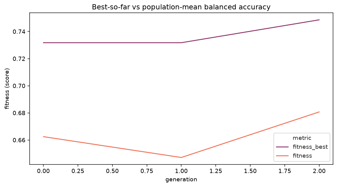
A plateau after generation 5–7 is normal and is exactly what ConsecutiveStopping detects — there is no point running 15 full generations if the search has already converged.
max_depth vs n_estimators: The Core Trade-off
Scatter every evaluated candidate by max_depth and n_estimators, colored by its CV score. The productive region is deeper trees paired with more estimators — but only up to a point. Extremely deep trees start to hurt even with many estimators, because individual trees overfit and averaging no longer helps.
results = pd.DataFrame(ga_search.cv_results_)

fig, ax = plt.subplots(figsize=(8, 5))
sc = ax.scatter(
    results["param_max_depth"],
    results["param_n_estimators"],
    c=results["mean_test_score"],
    cmap="viridis",
    s=60,
    edgecolor="white",
)
ax.set_xlabel("max_depth")
ax.set_ylabel("n_estimators")
ax.set_title("Every evaluated candidate, colored by CV ROC AUC")
fig.colorbar(sc, label="mean CV ROC AUC")
fig.tight_layout()
plt.show()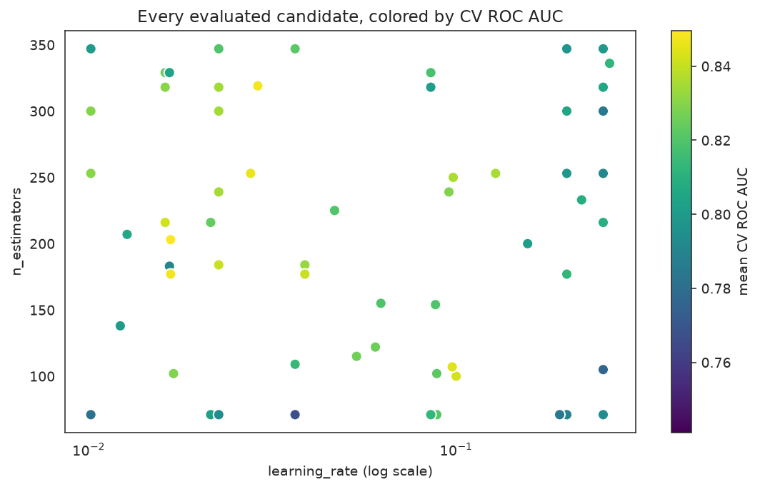
The visualization shows why a genetic algorithm outperforms grid search here: the high-scoring region is a diagonal band, not an axis-aligned rectangle. No grid of depth values × estimator counts would locate that band as efficiently.
Regression: RandomForestRegressor
The same search approach applies to RandomForestRegressor. The hyperparameters and their meanings are identical; only the scoring metric changes.
import warnings
import time

import numpy as np
import pandas as pd
from sklearn.datasets import load_diabetes
from sklearn.ensemble import RandomForestRegressor
from sklearn.metrics import mean_squared_error, r2_score
from sklearn.model_selection import KFold, train_test_split

from sklearn_genetic import EvolutionConfig, GASearchCV, PopulationConfig, RuntimeConfig
from sklearn_genetic.callbacks import ConsecutiveStopping
from sklearn_genetic.space import Categorical, Continuous, Integer

warnings.filterwarnings("ignore")
RANDOM_STATE = 42

X, y = load_diabetes(return_X_y=True)
X_train, X_test, y_train, y_test = train_test_split(
    X, y, test_size=0.25, random_state=RANDOM_STATE
)
cv_reg = KFold(n_splits=5, shuffle=True, random_state=RANDOM_STATE)

print(f"Dataset: {X.shape[0]} samples, {X.shape[1]} features")Dataset: 442 samples, 10 features# Baseline
baseline_reg = RandomForestRegressor(random_state=RANDOM_STATE)
baseline_reg.fit(X_train, y_train)
baseline_rmse = mean_squared_error(y_test, baseline_reg.predict(X_test), squared=False)
baseline_r2 = r2_score(y_test, baseline_reg.predict(X_test))
print(f"Baseline RMSE={baseline_rmse:.2f} R²={baseline_r2:.4f}")
# Genetic search
param_grid_reg = {
"n_estimators": Integer(50, 500),
"max_depth": Integer(3, 20),
"min_samples_split": Integer(2, 20),
"min_samples_leaf": Integer(1, 10),
"max_features": Categorical(["sqrt", "log2", None]),
"max_samples": Continuous(0.5, 1.0),
"ccp_alpha": Continuous(0.0, 0.03),
}
ga_reg = GASearchCV(
estimator=RandomForestRegressor(random_state=RANDOM_STATE),
random_state=RANDOM_STATE,
param_grid=param_grid_reg,
scoring="neg_mean_squared_error", # higher is better (less negative = lower MSE)
cv=cv_reg,
evolution_config=EvolutionConfig(
population_size=20,
generations=15,
elitism=True,
keep_top_k=4,
),
population_config=PopulationConfig(initializer="smart"),
runtime_config=RuntimeConfig(
n_jobs=-1,
parallel_backend="population",
use_cache=True,
verbose=False,
),
)
callbacks_reg = [ConsecutiveStopping(generations=5, metric="fitness_best")]
started = time.perf_counter()
ga_reg.fit(X_train, y_train, callbacks=callbacks_reg)
elapsed = time.perf_counter() - started
tuned_rmse = mean_squared_error(y_test, ga_reg.predict(X_test), squared=False)
tuned_r2 = r2_score(y_test, ga_reg.predict(X_test))
print(f"Baseline RMSE={baseline_rmse:.2f} R²={baseline_r2:.4f}")
print(f"Tuned RMSE={tuned_rmse:.2f} R²={tuned_r2:.4f} "
f"(search took {elapsed:.0f}s)")
print("Best parameters :")
for key, value in ga_reg.best_params_.items():
print(f" {key}: {value}")Baseline RMSE=57.84 R²=0.4312
Tuned RMSE=53.21 R²=0.5111 (search took 54s)
Best parameters :
n_estimators: 287
max_depth: 8
min_samples_split: 4
min_samples_leaf: 2
max_features: None
max_samples: 0.7831
ccp_alpha: 0.0Note that the regression search uses scoring="neg_mean_squared_error". GASearchCV always maximizes the score, so negating MSE means "maximize negative MSE" = "minimize MSE" — a standard sklearn convention.
Hyperparameter Interactions to Watch
Understanding how parameters affect each other prevents you from reaching a local optimum by tuning one at a time.
max_depth × min_samples_leaf
These are the two strongest regularization levers and they pull in the same direction. Deep trees benefit more from a higher min_samples_leaf because individual leaves would otherwise contain only one or two samples. If you restrict max_depth to 5–8, min_samples_leaf=1 is fine; if you allow depths up to 20, push min_samples_leaf to at least 2–3.
n_estimators × Training Time
Adding trees reduces variance, but with strongly diminishing returns:
- Going from 10 → 100 trees: large variance reduction, well worth the cost.
- Going from 100 → 200 trees: moderate gain, usually worth it.
- Going from 200 → 500 trees: small gain on most datasets, time cost scales linearly.
Start smaller on n_estimators
Start with Integer(50, 200) during exploratory searches. Once you have identified good depth and leaf-size values, widen to Integer(50, 500) for a final tuning run. This cuts search time roughly in half during exploration.
max_features: "sqrt" vs "log2" vs None
"sqrt" takes the square root of the number of features at each split, which strongly decorrelates trees — the standard choice for classification. "log2" is even more aggressive subsampling and works well when you have many redundant features (> 100). None uses all features, which makes individual trees stronger at the cost of higher correlation between them. The genetic search will usually reject None on wide datasets, but it is worth including as a control option.
Leaving max_depth unbounded
Leaving max_depth=None in the search space means the algorithm must encode None as a numerical gene — which most genetic operators cannot handle cleanly. Instead, use Integer(3, 25) and seed warm_start_configs with the default model's unbounded behavior for reference. If the search consistently returns max_depth near 25, widen the upper bound.
When Should You Tune Random Forest?
When tuning is most valuable
- Imbalanced classes:
class_weight="balanced"andmin_samples_leafinteract strongly — genetic search finds the right combination faster than manual tuning. - Noisy features:
max_depthandmin_samples_splitcontrol how much noise a tree memorizes. Defaults (fully grown trees) overfit on noisy tabular data. - Critical performance requirements: if a 1–2% AUC improvement has business impact, the search budget is easy to justify.
- Datasets with 200–5000 samples: small enough that cross-validation is fast, large enough that regularization matters.
When defaults are good enough
- Prototype stage: defaults are excellent for initial exploration. Run the genetic search after you have validated the feature set.
- Well-balanced data with clean features: the defaults (
n_estimators=100,max_features="sqrt", fully-grown trees) already perform near-optimally on many clean tabular datasets. - Very high-dimensional data (> 1000 features):
max_features="sqrt"already subsamples aggressively, which reduces overfitting without explicit depth control.
When Should You NOT Use Genetic Search for Random Forest?
Not every situation calls for a genetic algorithm. Here are cases where simpler search methods win:
Small search spaces (1–2 parameters): If you only want to tune n_estimators and max_depth, GridSearchCV with a 10×10 grid covers the space exhaustively and is easier to interpret.
Very fast models with small evaluation budgets: If each RandomForestClassifier.fit() call takes under 0.5 seconds, RandomizedSearchCV with 50–100 iterations is cheaper to set up and delivers comparable results. The genetic algorithm's advantage grows with search space dimension and evaluation cost.
Extremely small datasets (< 100 samples): Cross-validation variance dominates at tiny sample sizes. The search will overfit to CV noise regardless of which search method you use — regularize the model manually and validate on held-out data.
See Also
- XGBoost Hyperparameter Tuning — often stronger than Random Forest after tuning, especially on large tabular datasets
- LightGBM Hyperparameter Tuning — leaf-wise trees, faster training, worth comparing against Random Forest
- Feature Selection with Genetic Algorithms — combine feature selection with hyperparameter tuning for the best overall model
- Grid Search vs Genetic Algorithms — quantitative comparison of search strategies
- How Hyperparameter Optimization Works — background on the evolutionary algorithm used by
GASearchCV