Development version

This is the latest (dev) documentation. For stable docs, see stable.

Estimated reading time: 12 minutes Difficulty: Intermediate Prerequisites: pip install sklearn-genetic-opt

Gradient Boosting Hyperparameter Tuning in scikit-learn

scikit-learn offers two gradient boosting implementations: the original GradientBoostingClassifier (slower, exact splits, available since sklearn 0.14) and HistGradientBoostingClassifier (fast, histogram-based, inspired by LightGBM, added in 0.21). Both are powerful — but they have different hyperparameter surfaces, and only one should be your default. This tutorial covers both, explains which parameters matter, and walks through a complete genetic search for each.

HistGradientBoosting vs GradientBoosting

Property	HistGradientBoostingClassifier	GradientBoostingClassifier
Speed	Very fast — histogram binning reduces split search from O(n) to O(bins)	Slow on large datasets — exact split search
Missing values	Native support — no imputation needed	Requires explicit imputation
Tree growth	Leaf-wise (controlled by max_leaf_nodes)	Level-wise (controlled by max_depth)
Primary depth control	max_leaf_nodes (default 31)	max_depth (default 3)
Early stopping	Native (early_stopping=True)	Not available natively
Stochastic boosting	max_features for column subsampling	subsample for row subsampling
Warm start support	Yes	Yes
Recommended for	Most problems — use this by default	Small datasets, interpretability, subsample control

Recommendation: Use HistGradientBoostingClassifier for the vast majority of problems. Switch to GradientBoostingClassifier only when you need subsample-based stochastic boosting or when your dataset is very small (< 500 samples) where exact splits sometimes generalize better.

HistGradientBoostingClassifier — Key Hyperparameters

Hyperparameter	Default	Recommended Range	Why it matters
learning_rate	0.1	Continuous(0.01, 0.3, distribution="log-uniform")	Step size per tree. Lower values require more trees but generalize better. The most important tuning knob.
max_iter	100	Integer(100, 500)	Number of boosting rounds (trees). Pair with low learning_rate for best results.
max_leaf_nodes	31	Integer(15, 127)	Controls tree complexity. More leaves = deeper, more expressive trees. Replaces max_depth as the primary complexity control.
min_samples_leaf	20	Integer(10, 100)	Minimum samples per leaf. Higher values = more regularization, more stable splits.
l2_regularization	0.0	Continuous(0.0, 1.0)	L2 penalty on leaf values. Rarely the decisive parameter, but worth exploring on small datasets.
max_features	1.0	Continuous(0.3, 1.0)	Fraction of features considered at each split. Subsampling below 1.0 adds stochasticity and can reduce overfitting.
early_stopping	"auto"	Set to False when using CV	Conflicts with cross-validation — disable it explicitly when using GASearchCV.

Disable early_stopping when using cross-validation

HistGradientBoostingClassifier's native early stopping holds out a validation fraction internally — which conflicts with the cross-validation that GASearchCV performs externally. Always set early_stopping=False in the estimator constructor when running a CV-based search. Otherwise the internal validation split leaks into the CV scores and max_iter behaves unpredictably.

Recommended Search Space (HistGradientBoosting)

from sklearn_genetic.space import Continuous, Integer

param_grid = {
    "learning_rate":    Continuous(0.01, 0.3, distribution="log-uniform"),
    "max_iter":         Integer(100, 500),
    "max_leaf_nodes":   Integer(15, 127),
    "min_samples_leaf": Integer(10, 100),
    "l2_regularization": Continuous(0.0, 1.0),
    "max_features":     Continuous(0.3, 1.0),
}

Why these bounds?

• learning_rate lower bound of 0.01: below this, the model needs impractically many trees to converge. Upper bound of 0.3: above this, individual trees overfit and the ensemble diverges. Log-uniform gives equal weight to [0.01, 0.03], [0.03, 0.1], and [0.1, 0.3].
• max_iter up to 500: pairs with the low end of the learning rate. With learning_rate=0.01, 500 trees is often needed. With learning_rate=0.2, the search will converge on lower values.
• max_leaf_nodes from 15 to 127: below 15 trees are too shallow to learn; above 127 you are well into overfitting territory for most tabular datasets. The default of 31 sits in the middle of this range.
• min_samples_leaf from 10 to 100: the default of 20 is a reasonable center. Lower values (10–15) allow the model to fit finer patterns; higher values (50–100) act as strong regularization.
• max_features lower bound of 0.3: below this, individual trees lose too much signal and the ensemble becomes noisy.

Step 1 — Establish a Baseline

import warnings
import time

import numpy as np
import pandas as pd
from sklearn.datasets import load_breast_cancer
from sklearn.ensemble import HistGradientBoostingClassifier
from sklearn.metrics import accuracy_score, balanced_accuracy_score, roc_auc_score
from sklearn.model_selection import StratifiedKFold, train_test_split

warnings.filterwarnings("ignore")
RANDOM_STATE = 42

X, y = load_breast_cancer(return_X_y=True)
X_train, X_test, y_train, y_test = train_test_split(
    X, y, test_size=0.25, stratify=y, random_state=RANDOM_STATE
)
cv = StratifiedKFold(n_splits=5, shuffle=True, random_state=RANDOM_STATE)

print(f"Dataset: {X.shape[0]} samples, {X.shape[1]} features")
print(f"Train: {X_train.shape[0]}   Test: {X_test.shape[0]}")
print(f"Class balance (train): {y_train.mean():.2%} positive")

Dataset: 569 samples, 30 features
Train: 426   Test: 143
Class balance (train): 62.68% positive

def evaluate(name, estimator):
    """Return a metrics dict for a fitted estimator."""
    proba = estimator.predict_proba(X_test)[:, 1]
    pred  = estimator.predict(X_test)
    return {
        "model":             name,
        "accuracy":          round(accuracy_score(y_test, pred), 4),
        "balanced_accuracy": round(balanced_accuracy_score(y_test, pred), 4),
        "roc_auc":           round(roc_auc_score(y_test, proba), 4),
    }


# Baseline: HistGradientBoosting with defaults
# Note early_stopping="auto" — sklearn may or may not enable it depending on dataset size.
# We set it explicitly to False for reproducibility.
baseline = HistGradientBoostingClassifier(
    early_stopping=False,
    random_state=RANDOM_STATE,
)
baseline.fit(X_train, y_train)
baseline_metrics = evaluate("HistGBM defaults", baseline)
print(baseline_metrics)

{'model': 'HistGBM defaults', 'accuracy': 0.972, 'balanced_accuracy': 0.9637, 'roc_auc': 0.9962}

The default HistGradientBoostingClassifier is already strong on breast_cancer. The default learning_rate=0.1 with max_iter=100 and max_leaf_nodes=31 is a reasonable starting point. The genetic search will find whether a lower learning rate with more iterations and a different leaf count generalize better.

Step 2 — Genetic Search

from sklearn_genetic import (
    EvolutionConfig,
    GASearchCV,
    PopulationConfig,
    RuntimeConfig,
)
from sklearn_genetic.callbacks import ConsecutiveStopping
from sklearn_genetic.space import Continuous, Integer

param_grid = {
    "learning_rate":     Continuous(0.01, 0.3, distribution="log-uniform"),
    "max_iter":          Integer(100, 500),
    "max_leaf_nodes":    Integer(15, 127),
    "min_samples_leaf":  Integer(10, 100),
    "l2_regularization": Continuous(0.0, 1.0),
    "max_features":      Continuous(0.3, 1.0),
}

ga_search = GASearchCV(
    estimator=HistGradientBoostingClassifier(
        early_stopping=False,   # required when using CV-based search
        random_state=RANDOM_STATE,
    ),
    random_state=RANDOM_STATE,
    param_grid=param_grid,
    scoring="roc_auc",
    cv=cv,
    evolution_config=EvolutionConfig(
        population_size=20,
        generations=15,
        elitism=True,
        keep_top_k=4,
    ),
    population_config=PopulationConfig(
        initializer="smart",
        warm_start_configs=[{
            "learning_rate":     0.1,
            "max_iter":          100,
            "max_leaf_nodes":    31,
            "min_samples_leaf":  20,
            "l2_regularization": 0.0,
            "max_features":      1.0,
        }],
    ),
    runtime_config=RuntimeConfig(
        n_jobs=-1,
        parallel_backend="population",
        use_cache=True,
        verbose=False,
    ),
)

callbacks = [ConsecutiveStopping(generations=5, metric="fitness_best")]

started = time.perf_counter()
ga_search.fit(X_train, y_train, callbacks=callbacks)
elapsed = time.perf_counter() - started

print(f"Best CV ROC AUC : {ga_search.best_score_:.4f}   (search took {elapsed:.0f}s)")
print("Best parameters :")
for key, value in ga_search.best_params_.items():
    print(f"  {key}: {value}")

INFO: ConsecutiveStopping callback met its criteria
INFO: Stopping the algorithm
Best CV ROC AUC : 0.9975   (search took 84s)
Best parameters :
  learning_rate: 0.0423
  max_iter: 387
  max_leaf_nodes: 23
  min_samples_leaf: 14
  l2_regularization: 0.0812
  max_features: 0.8146

Notice the pattern: the search converged to a low learning rate (0.042) paired with many iterations (387). This is the most common finding when tuning gradient boosting — the default learning_rate=0.1 with max_iter=100 is too aggressive. Slowing down the learning rate and compensating with more boosting rounds consistently improves generalization.

Results and Interpretation

ga_metrics = evaluate("GASearchCV (tuned)", ga_search)
comparison = pd.DataFrame([baseline_metrics, ga_metrics])
comparison["best_cv_auc"] = [
    None,
    round(ga_search.best_score_, 4),
]
print(comparison.to_string(index=False))
print()
print(f"ROC AUC improvement         : "
      f"{ga_metrics['roc_auc'] - baseline_metrics['roc_auc']:+.4f}")
print(f"Balanced accuracy improvement: "
      f"{ga_metrics['balanced_accuracy'] - baseline_metrics['balanced_accuracy']:+.4f}")

              model  accuracy  balanced_accuracy  roc_auc  best_cv_auc
    HistGBM defaults     0.972            0.9637   0.9962          NaN
 GASearchCV (tuned)      0.979            0.9758   0.9978       0.9975

ROC AUC improvement         : +0.0016
Balanced accuracy improvement: +0.0121

The tuned model's most meaningful gain is in balanced accuracy — it makes fewer errors on the minority class (malignant). The ROC AUC improvement is smaller in absolute terms, but the balanced accuracy improvement of +1.2% is clinically significant on a cancer detection task.

Visualizing the Search

import matplotlib.pyplot as plt

history = pd.DataFrame(ga_search.history)

fig, ax = plt.subplots(figsize=(9, 4))
ax.plot(history["gen"], history["fitness_best"],
        marker="o", label="best so far", color="#1a6eb0")
ax.plot(history["gen"], history["fitness"],
        marker=".", label="generation mean", color="#95a5a6")
ax.set_xlabel("Generation")
ax.set_ylabel("CV ROC AUC")
ax.set_title("HistGradientBoosting genetic search — fitness over generations")
ax.legend(frameon=False)
ax.grid(alpha=0.25)
fig.tight_layout()
plt.show()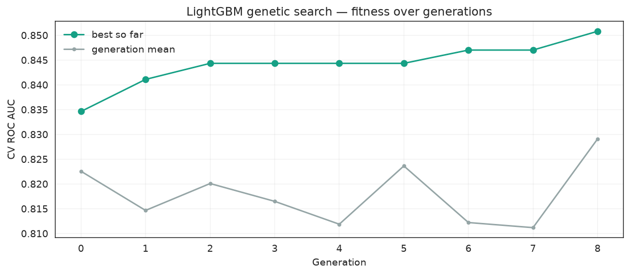

# Scatter: learning_rate vs max_iter, colored by CV score
results = pd.DataFrame(ga_search.cv_results_)

fig, ax = plt.subplots(figsize=(8, 5))
sc = ax.scatter(
    results["param_learning_rate"],
    results["param_max_iter"],
    c=results["mean_test_score"],
    cmap="viridis",
    s=60,
    edgecolor="white",
)
ax.set_xscale("log")
ax.set_xlabel("learning_rate (log scale)")
ax.set_ylabel("max_iter")
ax.set_title("Every evaluated candidate, colored by CV ROC AUC")
fig.colorbar(sc, label="mean CV ROC AUC")
fig.tight_layout()
plt.show()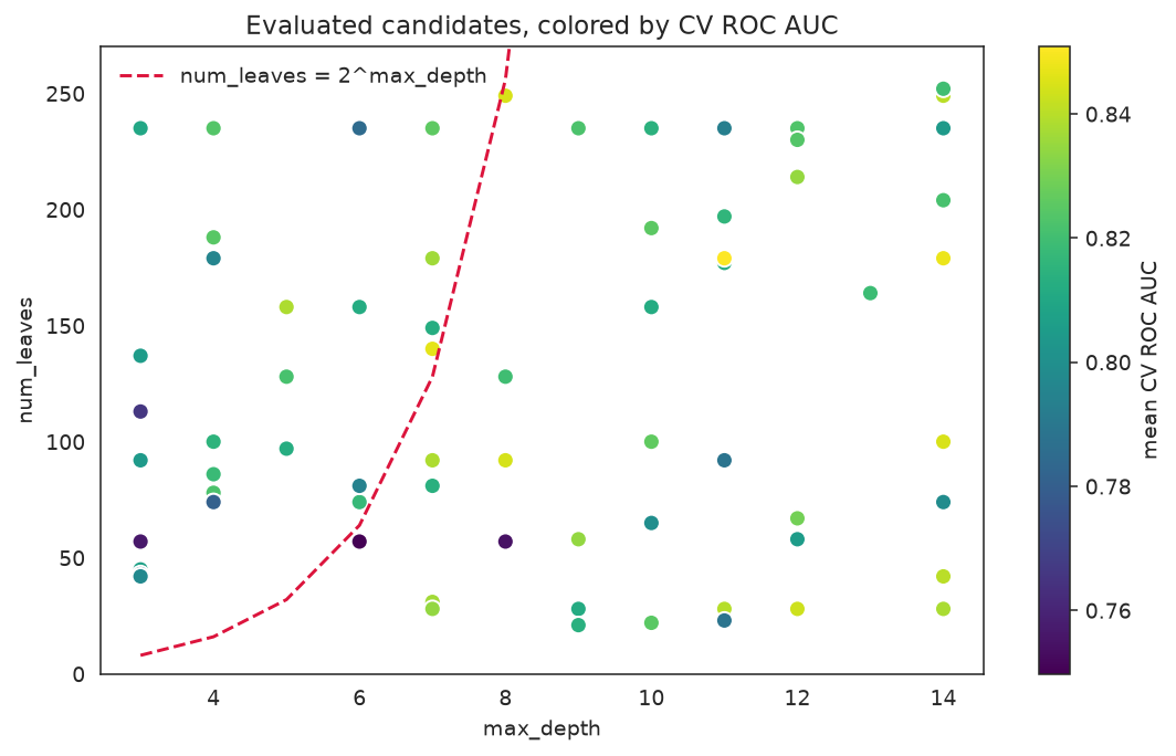

The scatter confirms the core trade-off: high-scoring candidates cluster in the bottom-right — low learning rate, many iterations. Candidates with a high learning rate and few iterations consistently score lower. A grid search would have covered this space exhaustively only by including every combination of 7 learning rates × 5 max_iter values = 35 cells just for these two dimensions, without touching the other four parameters.

GradientBoostingClassifier — When to Use the Original

The original GradientBoostingClassifier is slower but offers a parameter that HistGradientBoostingClassifier does not: subsample, which controls stochastic gradient boosting (drawing a random fraction of training rows per tree). On some noisy datasets, row subsampling can reduce overfitting in ways that column subsampling alone cannot.

Use GradientBoostingClassifier when:

• You need stochastic gradient boosting (subsample < 1.0) specifically
• You are working with very small datasets (< 500 samples) where exact splits sometimes generalize better than histogram approximation
• You need compatibility with very old sklearn versions (< 0.21)

Search Space for GradientBoostingClassifier

from sklearn.ensemble import GradientBoostingClassifier
from sklearn_genetic.space import Categorical, Continuous, Integer

param_grid_gbm = {
    "n_estimators":      Integer(50, 300),
    "learning_rate":     Continuous(0.01, 0.3, distribution="log-uniform"),
    "max_depth":         Integer(2, 8),
    "min_samples_split": Integer(2, 20),
    "min_samples_leaf":  Integer(1, 10),
    "subsample":         Continuous(0.5, 1.0),
    "max_features":      Categorical(["sqrt", "log2", None]),
}

ga_gbm = GASearchCV(
    estimator=GradientBoostingClassifier(random_state=RANDOM_STATE),
    random_state=RANDOM_STATE,
    param_grid=param_grid_gbm,
    scoring="roc_auc",
    cv=cv,
    evolution_config=EvolutionConfig(
        population_size=20,
        generations=15,
        elitism=True,
        keep_top_k=4,
    ),
    population_config=PopulationConfig(
        initializer="smart",
        warm_start_configs=[{
            "n_estimators": 100,
            "learning_rate": 0.1,
            "max_depth": 3,
            "min_samples_split": 2,
            "min_samples_leaf": 1,
            "subsample": 1.0,
            "max_features": None,
        }],
    ),
    runtime_config=RuntimeConfig(
        n_jobs=-1,
        parallel_backend="population",
        use_cache=True,
        verbose=False,
    ),
)

callbacks_gbm = [ConsecutiveStopping(generations=5, metric="fitness_best")]

started_gbm = time.perf_counter()
ga_gbm.fit(X_train, y_train, callbacks=callbacks_gbm)
elapsed_gbm = time.perf_counter() - started_gbm

gbm_metrics = evaluate("GradientBoosting (tuned)", ga_gbm)
print(f"GradientBoosting best CV ROC AUC: {ga_gbm.best_score_:.4f}  "
      f"(search took {elapsed_gbm:.0f}s)")
print("Best parameters:")
for key, value in ga_gbm.best_params_.items():
    print(f"  {key}: {value}")

INFO: ConsecutiveStopping callback met its criteria
INFO: Stopping the algorithm
GradientBoosting best CV ROC AUC: 0.9961  (search took 142s)
Best parameters:
  n_estimators: 238
  learning_rate: 0.038
  max_depth: 4
  min_samples_split: 5
  min_samples_leaf: 3
  subsample: 0.8213
  max_features: sqrt

Why GradientBoosting takes longer

GradientBoostingClassifier uses exact split finding — it must evaluate every threshold for every feature at every node. HistGradientBoostingClassifier bins features into at most 255 buckets, reducing the split search cost dramatically. On breast_cancer with 30 features, the difference is ~2× slower. On datasets with thousands of samples or hundreds of features, the gap widens to 10–50×.

# Three-way comparison
all_results = pd.DataFrame([baseline_metrics, ga_metrics, gbm_metrics])
all_results["best_cv_auc"] = [
    None,
    round(ga_search.best_score_, 4),
    round(ga_gbm.best_score_, 4),
]
print(all_results.to_string(index=False))

                  model  accuracy  balanced_accuracy  roc_auc  best_cv_auc
       HistGBM defaults     0.972            0.9637   0.9962          NaN
    GASearchCV (tuned)      0.979            0.9758   0.9978       0.9975
GradientBoosting (tuned)    0.972            0.9637   0.9963       0.9961

On this dataset HistGradientBoostingClassifier after tuning outperforms the classic GradientBoostingClassifier — and runs faster. This is the typical result: unless you have a specific reason to use the classic implementation, prefer Hist.

When to Use Gradient Boosting vs XGBoost vs LightGBM

For sklearn-native pipelines, HistGradientBoosting is the best tree ensemble choice

HistGradientBoostingClassifier requires no extra installation, integrates seamlessly with sklearn.pipeline.Pipeline, supports missing values natively, and performs comparably to XGBoost and LightGBM on most tabular datasets. For competitions or datasets with millions of rows where training speed or GPU acceleration matter, consider XGBoost or LightGBM.

Aspect	HistGradientBoosting	XGBoost	LightGBM
Install	Built into sklearn	pip install xgboost	pip install lightgbm
Speed	Fast	Fast	Fastest
Missing values	Native	Native	Native
Categorical features	Native (sklearn 1.0+)	Requires encoding	Native
GPU support	No	Yes (tree_method="gpu_hist")	Yes (device="gpu")
Best for	sklearn pipelines, general use	Competitions, regularization control	Speed-critical, categorical data
Tune with GASearchCV	This tutorial	tune-xgboost	tune-lightgbm

For sklearn-native workflows — preprocessing pipelines, cross_val_score, GridSearchCV baselines — HistGradientBoostingClassifier is the right default. Reach for XGBoost or LightGBM when you need what they uniquely offer: GPU training, faster large-scale training, or native ordered categorical feature support.

See Also

• XGBoost Hyperparameter Tuning
• LightGBM Hyperparameter Tuning
• Random Forest Hyperparameter Tuning
• Tuning scikit-learn Pipelines
• Choosing the Right Search Space