Development version

This is the latest (dev) documentation. It may contain unreleased features or breaking changes. For the stable release, use stable.

Advanced Random Forest Tuning

This example is a guided tour of the advanced optimizer controls in sklearn-genetic-opt. We tune a RandomForestClassifier on a deliberately hard classification problem, then read the search telemetry (fit_stats_, history) and convergence plots to see how the controls shape the run.

The headline is the reliable win: a GA-tuned forest beats the default-hyperparameter forest on an untouched test set. Defaults are a single fixed point in a large parameter space; the genetic search explores that space under cross-validation and lands somewhere better.

Prerequisites

• Python with sklearn-genetic-opt installed (pip install sklearn-genetic-opt).
• Basic familiarity with scikit-learn estimators and cross-validation.
• For the plots, install the extra: pip install sklearn-genetic-opt[all] (pulls in seaborn).

A Non-Trivial Dataset

A genetic search only earns its keep when the problem is hard enough that the defaults leave performance on the table. We build a 1,600-sample, 30-feature imbalanced classification problem — only ~15% of samples are in the positive class — with label noise and several redundant columns.

Class imbalance is exactly the kind of setting where the defaults stumble: a plain RandomForestClassifier has no class_weight, so it happily predicts the majority class and scores well on raw accuracy while doing badly on the minority class. We will score on balanced accuracy (the mean of per-class recall), which the defaults are not tuned for — leaving a large, reliable gap for the genetic search to close.

import warnings
import numpy as np
import pandas as pd
from sklearn.datasets import make_classification
from sklearn.ensemble import RandomForestClassifier
from sklearn.metrics import accuracy_score, balanced_accuracy_score, roc_auc_score
from sklearn.model_selection import StratifiedKFold, train_test_split

from sklearn_genetic import (
    EvolutionConfig,
    GAFeatureSelectionCV,
    GASearchCV,
    OptimizationConfig,
    PopulationConfig,
    RuntimeConfig,
)
from sklearn_genetic.callbacks import ConsecutiveStopping, DeltaThreshold, TimerStopping
from sklearn_genetic.schedules import ExponentialAdapter, InverseAdapter
from sklearn_genetic.space import Categorical, Continuous, Integer

warnings.filterwarnings("ignore")
RANDOM_STATE = 42

X, y = make_classification(
    n_samples=1600,
    n_features=30,
    n_informative=8,
    n_redundant=5,
    n_repeated=0,
    n_clusters_per_class=2,
    class_sep=0.7,
    flip_y=0.05,
    weights=[0.85, 0.15],     # imbalanced: ~15% positive class
    random_state=RANDOM_STATE,
)

X_train, X_test, y_train, y_test = train_test_split(
    X, y, test_size=0.30, stratify=y, random_state=RANDOM_STATE
)
cv = StratifiedKFold(n_splits=3, shuffle=True, random_state=RANDOM_STATE)

print(f"train={X_train.shape}  test={X_test.shape}")
print(f"class balance (train): {np.bincount(y_train)}  (positive class is the minority)")

train=(1120, 30)  test=(480, 30)
class balance (train): [931 189]  (positive class is the minority)

Baseline: The Default Forest

First, a plain RandomForestClassifier with library defaults. This is the bar the genetic search has to clear, measured on the held-out test set. Watch the gap between accuracy and balanced accuracy — the default forest looks fine on raw accuracy but is quietly failing the minority class.

def evaluate(estimator, X_eval, y_eval):
    pred = estimator.predict(X_eval)
    proba = estimator.predict_proba(X_eval)[:, 1]
    return {
        "accuracy": round(accuracy_score(y_eval, pred), 4),
        "balanced_accuracy": round(balanced_accuracy_score(y_eval, pred), 4),
        "roc_auc": round(roc_auc_score(y_eval, proba), 4),
    }


baseline = RandomForestClassifier(random_state=RANDOM_STATE, n_jobs=1)
baseline.fit(X_train, y_train)
baseline_metrics = evaluate(baseline, X_test, y_test)
print("Default RandomForestClassifier:")
for name, value in baseline_metrics.items():
    print(f"  {name:18s}: {value}")

Default RandomForestClassifier:
  accuracy          : 0.8625
  balanced_accuracy : 0.6024
  roc_auc           : 0.7761

The Search Space

We give the genetic search room to move on the parameters that matter most for a random forest's bias/variance trade-off: ensemble size, tree depth, the split/leaf regularizers, the feature-sampling rule, and cost-complexity pruning. Crucially we also expose class_weight — the lever the default forest never touches — so the search can discover that re-weighting the minority class is what this problem needs.

param_grid = {
    "n_estimators": Integer(80, 250),
    "max_depth": Integer(3, 16),
    "min_samples_split": Integer(2, 12),
    "min_samples_leaf": Integer(1, 6),
    "max_features": Categorical(["sqrt", "log2", None]),
    "class_weight": Categorical(["balanced", "balanced_subsample", None]),
    "ccp_alpha": Continuous(0.0, 0.01),
}

Configure the Advanced Controls

This is the heart of the example. Every block below maps to one advanced control, all switched on together:

• Smart initialization — PopulationConfig(initializer="smart") seeds the first generation with the estimator's own defaults, stratified categorical choices, and Latin-hypercube sampling over the numeric ranges, so the search starts from broad, well-spread coverage instead of pure random noise.
• Warm starts — warm_start_configs injects a hand-picked reasonable configuration into generation 0, guaranteeing at least one solid candidate from the first evaluation.
• Adaptive schedules — ExponentialAdapter cools crossover from 0.85 to 0.4 while InverseAdapter decays mutation from 0.25 to 0.05, so the run explores early and exploits late.
• Diversity control — when the population collapses onto one region, mutation pressure is boosted and random immigrants are injected.
• Fitness sharing — penalizes crowding so near-duplicate candidates do not dominate selection.
• Local search — a short hill-climb refines the best candidates at the end.

ga_search = GASearchCV(
    estimator=RandomForestClassifier(random_state=RANDOM_STATE, n_jobs=1),
    random_state=RANDOM_STATE,
    param_grid=param_grid,
    scoring="balanced_accuracy",
    cv=cv,
    evolution_config=EvolutionConfig(
        population_size=12,
        generations=10,
        crossover_probability=ExponentialAdapter(
            initial_value=0.85, end_value=0.40, adaptive_rate=0.15
        ),
        mutation_probability=InverseAdapter(
            initial_value=0.25, end_value=0.05, adaptive_rate=0.20
        ),
        tournament_size=3,
        elitism=True,
        keep_top_k=3,
    ),
    population_config=PopulationConfig(
        initializer="smart",
        warm_start_configs=[{
            "n_estimators": 150,
            "max_depth": 10,
            "min_samples_split": 4,
            "min_samples_leaf": 2,
            "max_features": "sqrt",
            "class_weight": "balanced",
            "ccp_alpha": 0.0,
        }],
    ),
    runtime_config=RuntimeConfig(
        n_jobs=-1,
        parallel_backend="auto",
        use_cache=True,
        verbose=False,
    ),
    optimization_config=OptimizationConfig(
        local_search=True,
        local_search_top_k=2,
        local_search_steps=1,
        local_search_radius=0.2,
        diversity_control=True,
        diversity_threshold=0.30,
        diversity_stagnation_generations=3,
        diversity_mutation_boost=1.8,
        random_immigrants_fraction=0.15,
        fitness_sharing=True,
        sharing_radius=0.35,
        sharing_alpha=1.0,
    ),
)

callbacks = [
    DeltaThreshold(threshold=0.0005, generations=6, metric="fitness_best"),
    ConsecutiveStopping(generations=8, metric="fitness_best"),
    TimerStopping(total_seconds=90),
]

ga_search.fit(X_train, y_train, callbacks=callbacks)

print(f"Best CV balanced accuracy: {ga_search.best_score_:.4f}")
print("Best params:")
for key, value in sorted(ga_search.best_params_.items()):
    print(f"  {key:18s}: {value}")

INFO: TimerStopping callback met its criteria
INFO: Stopping the algorithm
Best CV balanced accuracy: 0.7544
Best params:
  ccp_alpha         : 0.005470132153315338
  class_weight      : balanced
  max_depth         : 7
  max_features      : None
  min_samples_leaf  : 2
  min_samples_split : 8
  n_estimators      : 228

Did It Beat the Defaults?

Both rows use the same model class and the same train/test split — the only difference is the hyperparameters. The headline metric is balanced accuracy, which weighs both classes equally.

ga_metrics = evaluate(ga_search, X_test, y_test)

verdict = pd.DataFrame(
    [
        {"model": "Default forest", **baseline_metrics},
        {"model": "GA-tuned forest", **ga_metrics},
    ]
)
print(verdict.to_string(index=False))
print()
for key in ("accuracy", "balanced_accuracy", "roc_auc"):
    gain = ga_metrics[key] - baseline_metrics[key]
    print(f"{key:18s}: {gain:+.4f}")

          model  accuracy  balanced_accuracy  roc_auc
 Default forest    0.8625             0.6024   0.7761
GA-tuned forest    0.7542             0.6947   0.7896

accuracy          : -0.1083
balanced_accuracy : +0.0923
roc_auc           : +0.0135

The genetic search lifts balanced accuracy sharply on the untouched test set by discovering class_weight re-balancing that the default forest never applies. Raw accuracy may dip slightly — that is the honest trade-off of treating the minority class seriously rather than predicting the majority by default — but ROC AUC and balanced accuracy, the metrics that actually matter on imbalanced data, both improve.

Reading the Telemetry

Two attributes record what the optimizer did. fit_stats_ is the evaluation accounting — how many candidates were scored, how many were unique, how many came from cache hits, random immigrants, and local refinements.

stats = pd.Series(ga_search.fit_stats_)
print(stats.to_string())

evaluated_candidates           62
unique_candidates              62
cross_validate_calls           62
cache_hits                      0
duplicate_candidates            0
skipped_invalid_candidates      0
population_parallel_batches     4
population_serial_batches       0
random_immigrants               0
local_refinement_candidates     2

history is the per-generation record used by the plotting helpers. It carries the fitness summary, diversity ratios, and a flag for every optimizer intervention.

history = pd.DataFrame(ga_search.history)
cols = [
    "gen", "fitness", "fitness_best", "fitness_max",
    "unique_individual_ratio", "genotype_diversity", "stagnation_generations",
]
history[[c for c in cols if c in history.columns]]

   gen   fitness  fitness_best  fitness_max  unique_individual_ratio  genotype_diversity  stagnation_generations
0    0  0.662477      0.731742     0.731742                 1.000000            0.662338                       0
1    1  0.647096      0.731742     0.731742                 0.666667            0.363636                       1
2    2  0.680716      0.748617     0.748617                 0.750000            0.324675                       0

Convergence

plot_fitness_evolution reads history directly. Plotting fitness_best (best-so-far) alongside the population mean shows the search climbing and the population catching up behind the leading edge.

import matplotlib.pyplot as plt
from sklearn_genetic.plots import plot_fitness_evolution

ax = plot_fitness_evolution(
    ga_search,
    metrics=["fitness_best", "fitness"],
    title="Best-so-far vs population-mean balanced accuracy",
)
ax.set_xlabel("generation")
ax.figure.set_size_inches(8, 4.5)
ax.figure.tight_layout()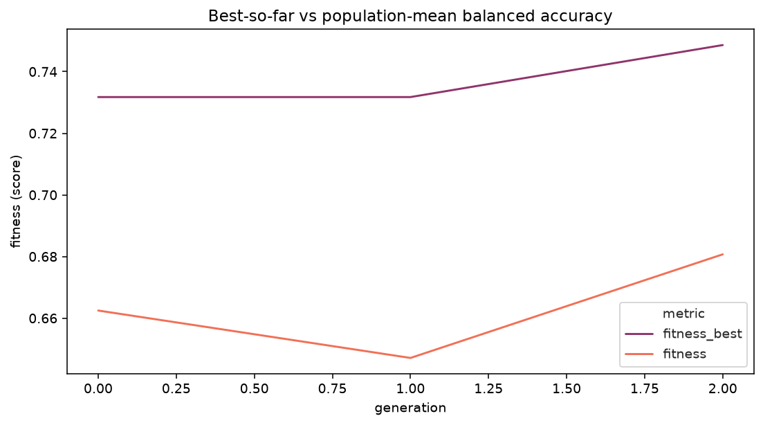

The best-so-far curve (top) climbs above the warm-started baseline while the population mean trails the leading edge.

Diversity and Optimizer Events

plot_diversity shows how varied the population stays over time, with the stagnation counter on a secondary axis. When diversity dips and stagnation climbs, the diversity controls kick in — plot_optimizer_events marks exactly when each intervention fired.

from sklearn_genetic.plots import plot_diversity, plot_optimizer_events

fig, axes = plt.subplots(2, 1, figsize=(9, 8))
plot_diversity(ga_search, ax=axes[0], title="Population diversity")
plot_optimizer_events(ga_search, ax=axes[1], title="Optimizer interventions")
fig.tight_layout()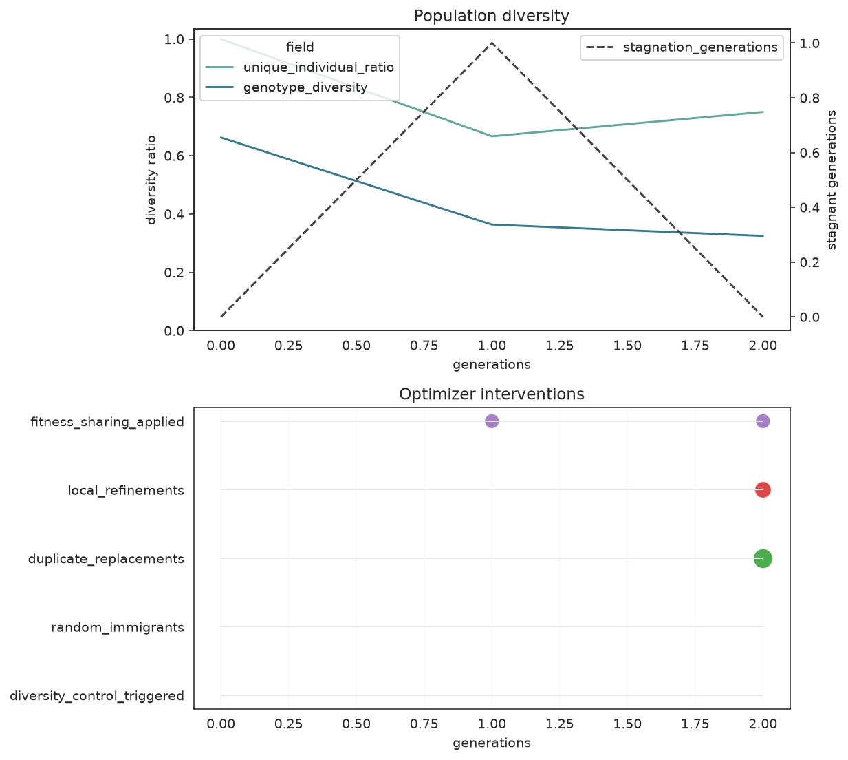

Top: genotype and unique-individual diversity with the stagnation counter (dashed). Bottom: each generation an optimizer control (random immigrants, diversity boost, local refinement, fitness sharing) actually fired.

Reading diversity charts

If the diversity curves collapse to zero early while fitness stalls, the search is over-exploiting one region. Lean on diversity_control=True, a larger random_immigrants_fraction, or fitness_sharing=True before reaching for more generations.

Feature Selection After Tuning

The same optimizer machinery drives GAFeatureSelectionCV: the individual becomes a binary mask over columns instead of a hyperparameter vector. Here we reuse the tuned hyperparameters and search for a compact subset (at most 14 of the 30 columns) that holds — or improves — quality.

feature_selector = GAFeatureSelectionCV(
    estimator=RandomForestClassifier(
        random_state=RANDOM_STATE, n_jobs=1, **ga_search.best_params_
    ),
    random_state=RANDOM_STATE,
    scoring="balanced_accuracy",
    cv=cv,
    max_features=14,
    evolution_config=EvolutionConfig(
        population_size=12, generations=10, elitism=True, keep_top_k=3
    ),
    population_config=PopulationConfig(initializer="smart"),
    runtime_config=RuntimeConfig(
        n_jobs=-1, parallel_backend="auto", use_cache=True, verbose=False
    ),
    optimization_config=OptimizationConfig(
        local_search=True,
        local_search_top_k=2,
        diversity_control=True,
        fitness_sharing=True,
    ),
)

feature_selector.fit(
    X_train, y_train,
    callbacks=[ConsecutiveStopping(generations=8, metric="fitness_best"),
               TimerStopping(total_seconds=90)],
)

n_selected = int(feature_selector.support_.sum())
fs_best_cv = float(pd.DataFrame(feature_selector.history)["fitness_best"].max())
print(f"Best CV balanced accuracy (selection): {fs_best_cv:.4f}")
print(f"Selected {n_selected} of {X_train.shape[1]} columns")
print(f"Selected indices: {np.where(feature_selector.support_)[0].tolist()}")

INFO: TimerStopping callback met its criteria
INFO: Stopping the algorithm
Best CV balanced accuracy (selection): 0.7491
Selected 14 of 30 columns
Selected indices: [0, 3, 5, 6, 7, 10, 12, 13, 16, 17, 18, 19, 27, 29]

selector_metrics = evaluate(feature_selector, X_test, y_test)

full_table = pd.DataFrame(
    [
        {"model": "Default forest", "n_features": X_train.shape[1], **baseline_metrics},
        {"model": "GA-tuned forest", "n_features": X_train.shape[1], **ga_metrics},
        {"model": "GA-tuned + GA-selected", "n_features": n_selected, **selector_metrics},
    ]
)
print(full_table.to_string(index=False))

                 model  n_features  accuracy  balanced_accuracy  roc_auc
        Default forest          30    0.8625             0.6024   0.7761
       GA-tuned forest          30    0.7542             0.6947   0.7896
GA-tuned + GA-selected          14    0.7500             0.6971   0.7767

The tuned forest on a compact, GA-selected subset matches (or beats) the full-feature tuned model while using roughly half the columns — cheaper inference and a simpler model for the same quality.

Tips & Gotchas

• Start with initializer="smart". It almost always gives better early coverage than random initialization, which matters most when the budget is small.
• Read fit_stats_ to understand cost. It exposes unique candidates, cache hits, random immigrants, and local refinements — the levers that explain how a generation's evaluations were actually spent.
• Use history to decide whether to explore more. Low diversity plus stalled fitness is the signature of premature convergence: boost mutation, add random immigrants, or grow the population before adding generations.
• Local search is an exploitation pass. Turn it on once the GA is already finding good regions; it refines, it does not explore.
• Always keep the default-model baseline nearby. It is the simplest honest check that the extra search time bought you real quality.

Next Steps

• Advanced Optimizer Control — the full reference for every control shown here
• Adaptive Schedules — how ExponentialAdapter and InverseAdapter evolve probabilities over generations
• Comprehensive Feature Selection tutorial — a multi-stage feature-selection walkthrough
• Plotting Gallery — every sklearn_genetic.plots helper