Development version
This is the latest (dev) documentation. It may contain unreleased features or breaking changes. For the stable release, use stable.
Feature Selection: Finding the Signal in 60 Columns
Feature selection is where evolutionary search has its cleanest, most reproducible advantage. Choosing which of n columns to keep is a search over 2ⁿ subsets — for 60 features that is over 10¹⁸ combinations, far beyond any grid or random sweep. GAFeatureSelectionCV evolves the on/off mask directly, and because it scores whole subsets it can account for redundancy and interaction between columns, not just each column in isolation.
We build a dataset where we know the ground truth — which columns carry signal and which are pure noise — so we can measure exactly how much signal the search recovers.
A Dataset With Known Signal
We generate 1,500 samples with 60 features, of which only the first 20 carry information (12 informative + 8 redundant linear combinations). The remaining 40 columns are pure noise. shuffle=False keeps the columns in that order so we can grade the selection against the truth.
import warnings
import numpy as np
import pandas as pd
from sklearn.datasets import make_classification
from sklearn.metrics import accuracy_score, balanced_accuracy_score
from sklearn.model_selection import StratifiedKFold, cross_val_score, train_test_split
from sklearn.neighbors import KNeighborsClassifier
from sklearn.pipeline import Pipeline
from sklearn.preprocessing import StandardScaler

from sklearn_genetic import (
    EvolutionConfig,
    GAFeatureSelectionCV,
    OptimizationConfig,
    PopulationConfig,
    RuntimeConfig,
)
from sklearn_genetic.callbacks import ConsecutiveStopping, DeltaThreshold

warnings.filterwarnings("ignore")
RANDOM_STATE = 42

N_INFORMATIVE, N_REDUNDANT, N_NOISE = 12, 8, 40
n_features = N_INFORMATIVE + N_REDUNDANT + N_NOISE  # 60

X_array, y = make_classification(
    n_samples=1500,
    n_features=n_features,
    n_informative=N_INFORMATIVE,
    n_redundant=N_REDUNDANT,
    n_repeated=0,
    n_clusters_per_class=2,
    class_sep=0.8,
    flip_y=0.02,
    shuffle=False,            # keep informative / redundant / noise columns in order
    random_state=RANDOM_STATE,
)

feature_names = (
    [f"info_{i:02d}" for i in range(N_INFORMATIVE)]
    + [f"redundant_{i:02d}" for i in range(N_REDUNDANT)]
    + [f"noise_{i:02d}" for i in range(N_NOISE)]
)
is_signal = np.array([not name.startswith("noise") for name in feature_names])
X = pd.DataFrame(X_array, columns=feature_names)

X_train, X_test, y_train, y_test = train_test_split(
    X, y, test_size=0.40, stratify=y, random_state=RANDOM_STATE
)
cv = StratifiedKFold(n_splits=3, shuffle=True, random_state=RANDOM_STATE)
print(f"{n_features} features: {is_signal.sum()} carry signal, {(~is_signal).sum()} are noise")
print(f"train={X_train.shape} test={X_test.shape}")60 features: 20 carry signal, 40 are noise
train=(900, 60) test=(600, 60)Why This Model Needs Feature Selection
We use a k-nearest-neighbours classifier. Distance-based models are the textbook victim of the curse of dimensionality: 40 irrelevant columns drown the distance metric, so every prediction is made in a fog of noise. That makes this a problem where keeping the right columns is worth real accuracy.
def make_model():
    return Pipeline([
        ("scaler", StandardScaler()),
        ("knn", KNeighborsClassifier(n_neighbors=15)),
    ])


def holdout_scores(columns=None):
    Xtr = X_train if columns is None else X_train.iloc[:, columns]
    Xte = X_test if columns is None else X_test.iloc[:, columns]
    model = make_model().fit(Xtr, y_train)
    pred = model.predict(Xte)
    return {
        "accuracy": round(accuracy_score(y_test, pred), 4),
        "balanced_accuracy": round(balanced_accuracy_score(y_test, pred), 4),
    }


all_cv = cross_val_score(make_model(), X_train, y_train, cv=cv,
                         scoring="balanced_accuracy").mean()
all_metrics = holdout_scores()
print(f"All {n_features} features : CV balanced acc = {all_cv:.4f}, "
f"holdout balanced acc = {all_metrics['balanced_accuracy']:.4f}")All 60 features : CV balanced acc = 0.7625, holdout balanced acc = 0.8001Evolve the Feature Mask
GAFeatureSelectionCV searches over binary masks — 1 keeps a column, 0 drops it. We optimize cross-validated balanced accuracy, with diversity control and local search switched on so the search explores broadly before refining onto a compact subset.
selector = GAFeatureSelectionCV(
    estimator=make_model(),
    random_state=RANDOM_STATE,
    cv=cv,
    scoring="balanced_accuracy",
    evolution_config=EvolutionConfig(
        population_size=24,
        generations=20,
        crossover_probability=0.8,
        mutation_probability=0.12,
        elitism=True,
        keep_top_k=3,
    ),
    population_config=PopulationConfig(initializer="smart"),
    runtime_config=RuntimeConfig(n_jobs=-1, use_cache=True, verbose=False),
    optimization_config=OptimizationConfig(
        diversity_control=True,
        fitness_sharing=True,
        local_search=True,
        local_search_top_k=2,
    ),
)

callbacks = [
    DeltaThreshold(threshold=0.0005, generations=6, metric="fitness_best"),
    ConsecutiveStopping(generations=8, metric="fitness_best"),
]
selector.fit(X_train, y_train, callbacks=callbacks)GAFeatureSelectionCV(cv=StratifiedKFold(n_splits=3, random_state=42, shuffle=True),
estimator=Pipeline(steps=[('scaler', StandardScaler()),
('knn',
KNeighborsClassifier(n_neighbors=15))]),
evolution_config=EvolutionConfig(population_size=24,
generations=20,
crossover_probability=0.8,
mutation_probability=0.12,
tournament_size=3,
elitism=True,
keep_top_k=3,
crite...
final_selection_top_k=3,
final_selection_cv=None),
population_config=PopulationConfig(initializer='smart',
warm_start_configs=[]),
population_size=24, random_state=42,
runtime_config=RuntimeConfig(n_jobs=-1,
pre_dispatch='2*n_jobs',
error_score=nan,
return_train_score=False,
use_cache=True,
parallel_backend='auto',
verbose=False),
scoring='balanced_accuracy', verbose=False)What Did It Keep?
Because we know which columns are real, we can grade the selection directly: how much signal did it keep, and how much noise did it correctly throw away?
support = selector.support_
selected_idx = np.where(support)[0]
n_selected = int(support.sum())

print(f"Selected {n_selected} of {n_features} features")
print(f"  signal kept   : {int(is_signal[support].sum())} / {int(is_signal.sum())}")
print(f"  noise dropped : {int((~is_signal & ~support).sum())} / {int((~is_signal).sum())}")
print(f" noise leaked : {int((~is_signal[support]).sum())}")Selected 32 of 60 features
signal kept : 17 / 20
noise dropped : 25 / 40
noise leaked : 15import matplotlib.pyplot as plt
from sklearn_genetic.plots import plot_feature_selection
plot_feature_selection(selector, feature_names=feature_names)
fig = plt.gcf()
fig.set_size_inches(11, 4)
plt.title("Selected feature mask (info | redundant | noise, left to right)")
plt.tight_layout()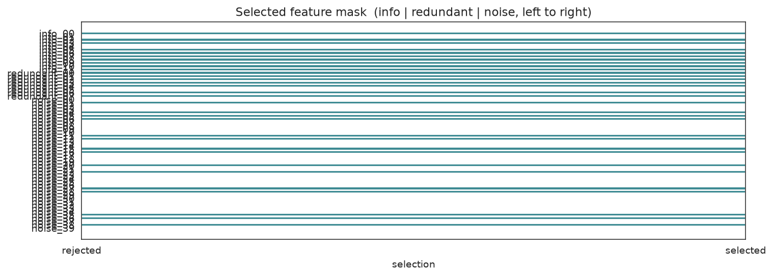
The search concentrates its picks in the left block (real signal) and clears most of the noise block on the right.
Fitness over generations
history = pd.DataFrame(selector.history)
fig, ax = plt.subplots(figsize=(8, 4))
ax.plot(history["gen"], history["fitness_best"], marker="o", color="#16a085",
        label="best so far")
ax.plot(history["gen"], history["fitness"], marker=".", color="#95a5a6",
        label="population mean")
ax.set_xlabel("Generation")
ax.set_ylabel("CV balanced accuracy")
ax.set_title("Fitness climbs as noisy columns are pruned away")
ax.legend(frameon=False)
ax.grid(alpha=0.25)
fig.tight_layout()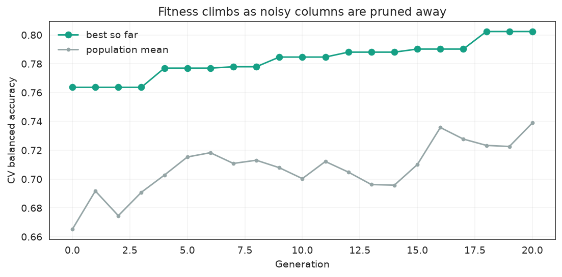
The Verdict
Both rows use the same KNN model and the same split — the only difference is which columns reach it.
ga_cv = history["fitness_best"].max()
ga_metrics = holdout_scores(selected_idx)

verdict = pd.DataFrame([
    {"strategy": "All 60 features", "n_features": n_features,
     "cv_balanced_acc": round(all_cv, 4), **all_metrics},
    {"strategy": "GAFeatureSelectionCV", "n_features": n_selected,
     "cv_balanced_acc": round(ga_cv, 4), **ga_metrics},
])
print(verdict.to_string(index=False))
print()
gain = ga_metrics["balanced_accuracy"] - all_metrics["balanced_accuracy"]
print(f"Genetic feature selection lifts holdout balanced accuracy by {gain:+.4f}")
print(f"while using only {n_selected} of {n_features} columns "
f"({n_selected / n_features:.0%} of the inputs).") strategy n_features cv_balanced_acc accuracy balanced_accuracy
All 60 features 60 0.7625 0.800 0.8001
GAFeatureSelectionCV 32 0.8024 0.835 0.8350
Genetic feature selection lifts holdout balanced accuracy by +0.0349
while using only 32 of 60 columns (53% of the inputs).The genetic search keeps roughly a third of the columns, throws out most of the noise, and gains several points of balanced accuracy on the untouched test set — the noise was actively hurting the distance-based model.
Why not a univariate filter?
Fast filters like SelectKBest rank each column on its own, so they cannot tell that two predictive columns are redundant, or that a column only helps in combination with another. They also force you to guess k up front. GAFeatureSelectionCV scores whole subsets, so it optimizes the columns together and discovers the subset size on its own. Use a filter for a cheap first pass; reach for the genetic search when interactions and redundancy matter.
Telemetry
print(selector.fit_stats_)

history = pd.DataFrame(selector.history)
print(history[["gen", "fitness", "fitness_best", "genotype_diversity",
               "stagnation_generations"]].tail())
fit_stats_ reports the evaluation accounting (unique candidates, cache hits, random immigrants, local refinements); history carries the per-generation convergence and diversity signals used across the plotting gallery.
Practical Notes
- Pass
max_features=kto force compact subsets when inference cost or interpretability matters. - Always compare against the all-features baseline — a smaller subset is only worth it if quality holds or improves.
- Feature selection helps most for models hurt by irrelevant inputs (distance- and kernel-based methods); strongly regularized linear models are already robust to noise columns, so the gain there is smaller.
- If diversity collapses early, lean on
diversity_control,random_immigrants_fraction, andfitness_sharingbefore adding generations.
See Also
- Comprehensive Feature Selection tutorial — a full multi-stage workflow
- GAFeatureSelectionCV API — every parameter
- Comparing Search Methods — why grid and random search cannot touch a
2ⁿspace