Development version

This is the latest (dev) documentation. It may contain unreleased features or breaking changes. For the stable release, use stable.

Basic Usage

This page walks through the two workflows you will use most:

• Hyperparameter tuning with GASearchCV
• Feature selection with GAFeatureSelectionCV

Every code block below is executed to build this page, so what you copy is exactly what ran — including the outputs and figures.

Prerequisites

• sklearn-genetic-opt installed (pip install sklearn-genetic-opt)
• Optional plotting extra for the figures: pip install sklearn-genetic-opt[plot]
• Basic familiarity with scikit-learn's fit / predict API

Hyperparameter Tuning

We tune an MLPClassifier on the handwritten digits dataset (10 classes, 64 pixel features). First, the imports and data:

import numpy as np
from sklearn.datasets import load_digits
from sklearn.metrics import accuracy_score
from sklearn.model_selection import StratifiedKFold, train_test_split
from sklearn.neural_network import MLPClassifier

from sklearn_genetic import EvolutionConfig, GASearchCV, PopulationConfig, RuntimeConfig
from sklearn_genetic.space import Categorical, Continuous, Integer

RANDOM_STATE = 42

X, y = load_digits(return_X_y=True)
X_train, X_test, y_train, y_test = train_test_split(
    X, y, test_size=0.33, stratify=y, random_state=RANDOM_STATE
)
cv = StratifiedKFold(n_splits=3, shuffle=True, random_state=RANDOM_STATE)
print(f"train={X_train.shape}  test={X_test.shape}  classes={len(np.unique(y))}")

train=(1203, 64)  test=(594, 64)  classes=10

Define the search space

The keys in param_grid are estimator parameter names. Each value is a space the genetic algorithm samples from:

• Integer — whole numbers in a range
• Continuous — floats in a range (optionally distribution="log-uniform")
• Categorical — a fixed list of choices

param_grid = {
    "hidden_layer_sizes": Categorical([(32,), (64,), (32, 16)]),
    "alpha": Continuous(1e-5, 1e-1, distribution="log-uniform"),
    "learning_rate_init": Continuous(1e-4, 1e-1, distribution="log-uniform"),
    "activation": Categorical(["relu", "tanh"]),
    "batch_size": Integer(32, 256),
}

Configure and run the search

GASearchCV is configured with small config objects. EvolutionConfig controls the population and generations; PopulationConfig(initializer="smart") builds a diverse, well-spread starting population; RuntimeConfig controls parallelism and logging.

clf = MLPClassifier(max_iter=150, early_stopping=True, random_state=RANDOM_STATE)

search = GASearchCV(
    estimator=clf,
    random_state=RANDOM_STATE,
    cv=cv,
    scoring="accuracy",
    param_grid=param_grid,
    evolution_config=EvolutionConfig(population_size=8, generations=6),
    population_config=PopulationConfig(initializer="smart"),
    runtime_config=RuntimeConfig(n_jobs=-1, verbose=False),
)

search.fit(X_train, y_train)

print(f"Best CV accuracy : {search.best_score_:.4f}")
print(f"Best parameters  : {search.best_params_}")

Best CV accuracy : 0.9584
Best parameters  : {'hidden_layer_sizes': (64,), 'alpha': 0.00027470715996250945, 'learning_rate_init': 0.003590489008293675, 'activation': 'relu', 'batch_size': 70}

After fitting, GASearchCV behaves like any fitted scikit-learn estimator — it has already refit the best configuration on all of X_train:

y_pred = search.predict(X_test)
print(f"Holdout accuracy : {accuracy_score(y_test, y_pred):.4f}")

Holdout accuracy : 0.9579

Reading the evolution

Each generation is logged. Inspect the full history as a DataFrame — the columns explain how the population improved and how diverse it stayed:

Column	Meaning
gen	generation number
fitness	mean CV score in the generation
fitness_best	best CV score found so far
genotype_diversity	1.0 = diverse, 0.0 = converged
unique_individual_ratio	fraction of distinct configurations
stagnation_generations	consecutive generations without improvement

import pandas as pd

history = pd.DataFrame(search.history)
print(history[["gen", "fitness", "fitness_best", "genotype_diversity",
               "unique_individual_ratio", "stagnation_generations"]].to_string(index=False))

 gen  fitness  fitness_best  genotype_diversity  unique_individual_ratio  stagnation_generations
   0 0.753325      0.946800            0.685714                    1.000                       0
   1 0.932253      0.946800            0.485714                    0.875                       1
   2 0.943890      0.955112            0.314286                    0.750                       0
   3 0.945449      0.955112            0.371429                    0.750                       1
   4 0.948462      0.955112            0.314286                    0.750                       2
   5 0.951995      0.955112            0.314286                    0.750                       3
   6 0.953242      0.958437            0.228571                    0.625                       0

fit_stats_ summarizes what the search actually spent — useful for spotting wasted effort (e.g. many skipped_invalid_candidates):

for key, value in search.fit_stats_.items():
    print(f"{key}: {value}")

evaluated_candidates: 104
unique_candidates: 102
cross_validate_calls: 102
cache_hits: 2
duplicate_candidates: 0
skipped_invalid_candidates: 0
population_parallel_batches: 7
population_serial_batches: 0
random_immigrants: 0
local_refinement_candidates: 0

Visualize convergence

With the [plot] extra installed, plot_fitness_evolution shows the best score climbing over generations, and plot_search_overview gives a compact diagnostic dashboard.

import matplotlib.pyplot as plt
from sklearn_genetic.plots import plot_search_overview

plot_search_overview(search, top_k=6)
plt.tight_layout()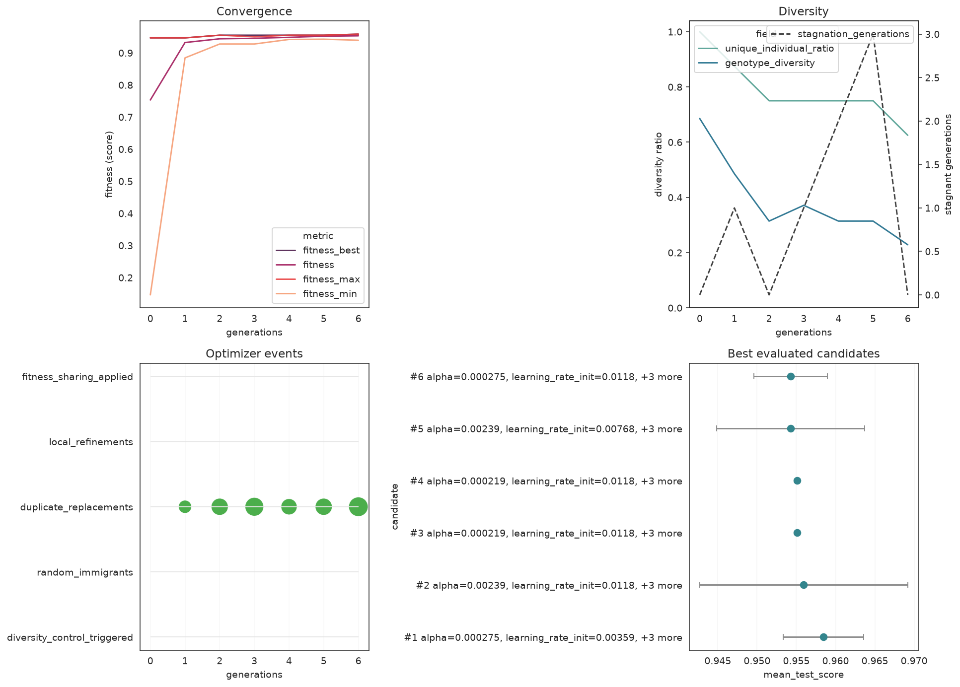

from sklearn_genetic.plots import plot_parameter_evolution

plot_parameter_evolution(search, parameters=["alpha", "learning_rate_init", "batch_size"])
plt.tight_layout()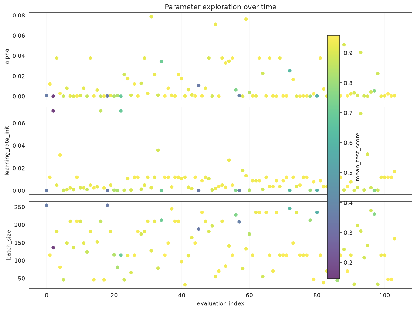

Feature Selection

GAFeatureSelectionCV searches for the most useful subset of columns. To make the task concrete we take the Iris dataset and bolt on 10 columns of pure noise; a good selector should keep the real measurements and discard the noise.

from sklearn.datasets import load_iris
from sklearn.svm import SVC

from sklearn_genetic import GAFeatureSelectionCV

iris = load_iris()
rng = np.random.default_rng(RANDOM_STATE)
noise = rng.uniform(0, 10, size=(iris.data.shape[0], 10))
X_fs = np.hstack([iris.data, noise])
feature_names = list(iris.feature_names) + [f"noise_{i}" for i in range(10)]
y_fs = iris.target

Xtr, Xte, ytr, yte = train_test_split(
    X_fs, y_fs, test_size=0.33, stratify=y_fs, random_state=RANDOM_STATE
)

selector = GAFeatureSelectionCV(
    estimator=SVC(gamma="auto"),
    random_state=RANDOM_STATE,
    cv=3,
    scoring="accuracy",
    evolution_config=EvolutionConfig(population_size=10, generations=8,
                                     elitism=True, keep_top_k=2),
    population_config=PopulationConfig(initializer="smart"),
    runtime_config=RuntimeConfig(n_jobs=-1, verbose=False),
)
selector.fit(Xtr, ytr)

selected = [name for name, keep in zip(feature_names, selector.support_) if keep]
print(f"Selected {len(selected)} of {len(feature_names)} features:")
for name in selected:
    print(f"  - {name}")
print(f"Holdout accuracy : {accuracy_score(yte, selector.predict(Xte)):.4f}")

Selected 3 of 14 features:
  - sepal length (cm)
  - sepal width (cm)
  - petal length (cm)
Holdout accuracy : 0.9800

support_ is a boolean mask (True = kept). The search keeps the informative Iris measurements and drops most of the noise columns. Visualize the mask:

from sklearn_genetic.plots import plot_feature_selection

plot_feature_selection(selector, feature_names=feature_names)
plt.tight_layout()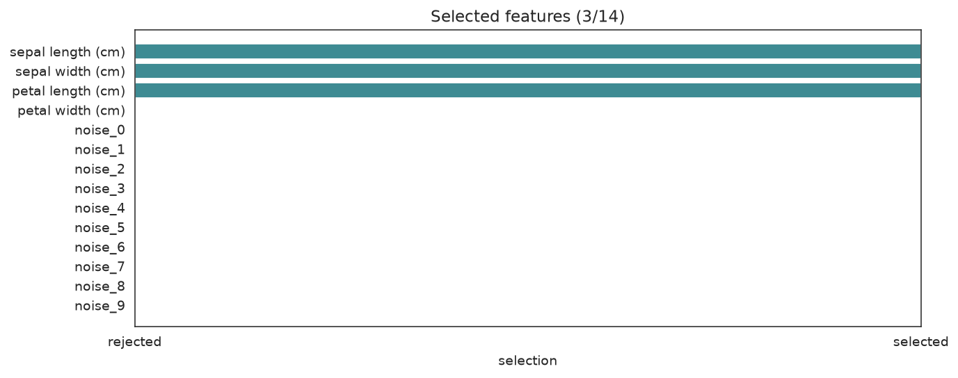

Tips & Gotchas

• Set RuntimeConfig(verbose=True) to watch the per-generation log live.
• PopulationConfig(initializer="smart") is strongly recommended — it usually finds better solutions faster than a purely random start.
• If accuracy is already near 1.0 on your data, switch to a more discriminative metric (e.g. roc_auc, balanced_accuracy).
• Check fit_stats_["skipped_invalid_candidates"] after fitting — a non-zero value means some sampled configurations raised errors during fit.

Next Steps

• When to Use — is a genetic search the right tool for your problem?
• Understanding Cross-Validation — read the generation log in depth
• Pipeline Tuning — tune a scikit-learn Pipeline with step__param names
• Callbacks — early stopping, progress bars, and checkpoints
• Plotting Gallery — every diagnostic plot, explained