Development version
This is the latest (dev) documentation. It may contain unreleased features or breaking changes. For the stable release, use stable.
Tuning XGBoost With GASearchCV
XGBoost has around nine hyperparameters that interact non-linearly: the right learning_rate depends on n_estimators, which depends on max_depth and the regularization terms. Out of the box, XGBoost's defaults (a high 0.3 learning rate, 100 deep trees) overfit noisy data. This tutorial searches the joint space with GASearchCV, shows the real gain over the default model, and visualizes the interaction the search exploits.
Prerequisites
pip install sklearn-genetic-opt xgboostA Dataset Where Defaults Overfit
We build a noisy binary problem — 30 features, only 8 informative, label noise, and overlapping clusters — so that an untuned, aggressive booster memorizes the training set instead of generalizing.
import warnings
import time

import numpy as np
import pandas as pd
from sklearn.datasets import make_classification
from sklearn.metrics import accuracy_score, balanced_accuracy_score, roc_auc_score
from sklearn.model_selection import StratifiedKFold, train_test_split
from xgboost import XGBClassifier

from sklearn_genetic import (
    EvolutionConfig,
    GASearchCV,
    OptimizationConfig,
    PopulationConfig,
    RuntimeConfig,
)
from sklearn_genetic.callbacks import ConsecutiveStopping, TimerStopping
from sklearn_genetic.schedules import ExponentialAdapter, InverseAdapter
from sklearn_genetic.space import Continuous, Integer

warnings.filterwarnings("ignore")
RANDOM_STATE = 42

X, y = make_classification(
    n_samples=2500,
    n_features=30,
    n_informative=8,
    n_redundant=8,
    n_clusters_per_class=3,
    class_sep=0.6,
    flip_y=0.08,
    random_state=RANDOM_STATE,
)
X_train, X_test, y_train, y_test = train_test_split(
    X, y, test_size=0.40, stratify=y, random_state=RANDOM_STATE
)
cv = StratifiedKFold(n_splits=3, shuffle=True, random_state=RANDOM_STATE)
print(f"train={X_train.shape} test={X_test.shape}")train=(1500, 30) test=(1000, 30)Baseline: XGBoost Defaults
XGBoost manages its own threads, so we set n_jobs=1 on the estimator and let sklearn-genetic-opt handle parallelism (see the note below).
def evaluate(name, estimator):
    proba = estimator.predict_proba(X_test)[:, 1]
    pred = estimator.predict(X_test)
    return {
        "model": name,
        "accuracy": round(accuracy_score(y_test, pred), 4),
        "balanced_accuracy": round(balanced_accuracy_score(y_test, pred), 4),
        "roc_auc": round(roc_auc_score(y_test, proba), 4),
    }


baseline = XGBClassifier(tree_method="hist", eval_metric="logloss",
                         random_state=RANDOM_STATE, n_jobs=1)
baseline.fit(X_train, y_train)
baseline_metrics = evaluate("XGBoost defaults", baseline)
print(baseline_metrics){'model': 'XGBoost defaults', 'accuracy': 0.794, 'balanced_accuracy': 0.794, 'roc_auc': 0.8608}The Search Space
Nine parameters with ranges grounded in XGBoost's documentation. log-uniform is used for parameters that matter across orders of magnitude, so each decade gets equal sampling probability instead of biasing toward large values.
param_grid = {
    "n_estimators":     Integer(50, 350),
    "max_depth":        Integer(2, 10),
    "min_child_weight": Integer(1, 12),
    "subsample":        Continuous(0.5, 1.0),
    "colsample_bytree": Continuous(0.4, 1.0),
    "learning_rate":    Continuous(0.01, 0.3, distribution="log-uniform"),
    "gamma":            Continuous(1e-4, 1.0, distribution="log-uniform"),
    "reg_alpha":        Continuous(1e-5, 10.0, distribution="log-uniform"),
    "reg_lambda":       Continuous(1e-5, 10.0, distribution="log-uniform"),
}
CPU oversubscription with XGBoost
XGBoost spawns threads internally for tree building. If the estimator uses n_jobs=-1 and the search parallelizes candidates, you get workers × xgb_threads threads — often several times your core count, which slows everything down. Pair n_jobs=1 on the XGBClassifier with parallel_backend="cv" so the search parallelizes at the fold level instead.
Configure and Run the Genetic Search
We keep the budget modest (a small population over a handful of generations) and let early stopping end it once progress stalls. warm_start_configs seeds the first population with XGBoost's defaults so the search starts from a known region; adaptive schedules anneal exploration into exploitation.
ga_search = GASearchCV(
    estimator=XGBClassifier(tree_method="hist", eval_metric="logloss",
                            random_state=RANDOM_STATE, n_jobs=1),
    random_state=RANDOM_STATE,
    param_grid=param_grid,
    scoring="roc_auc",
    cv=cv,
    evolution_config=EvolutionConfig(
        population_size=10,
        generations=8,
        crossover_probability=ExponentialAdapter(initial_value=0.8, end_value=0.4, adaptive_rate=0.15),
        mutation_probability=InverseAdapter(initial_value=0.25, end_value=0.05, adaptive_rate=0.20),
        tournament_size=3,
        elitism=True,
        keep_top_k=3,
    ),
    population_config=PopulationConfig(
        initializer="smart",
        warm_start_configs=[{
            "n_estimators": 100, "max_depth": 6, "min_child_weight": 1,
            "subsample": 0.8, "colsample_bytree": 0.8, "learning_rate": 0.1,
            "gamma": 1e-4, "reg_alpha": 1e-5, "reg_lambda": 1.0,
        }],
    ),
    runtime_config=RuntimeConfig(n_jobs=-1, parallel_backend="cv",
                                 use_cache=True, verbose=False),
    optimization_config=OptimizationConfig(
        diversity_control=True, fitness_sharing=True,
        local_search=True, local_search_top_k=2,
    ),
)

callbacks = [
    ConsecutiveStopping(generations=6, metric="fitness_best"),
    TimerStopping(total_seconds=90),
]
started = time.perf_counter()
ga_search.fit(X_train, y_train, callbacks=callbacks)
ga_seconds = time.perf_counter() - started

print(f"Best CV ROC AUC : {ga_search.best_score_:.4f}   (search took {ga_seconds:.0f}s)")
print("Best parameters :")
for key, value in ga_search.best_params_.items():
print(f" {key}: {value}")INFO: ConsecutiveStopping callback met its criteria
INFO: Stopping the algorithm
Best CV ROC AUC : 0.8497 (search took 41s)
Best parameters :
n_estimators: 203
max_depth: 7
min_child_weight: 3
subsample: 0.7600155334780292
colsample_bytree: 0.7095337198803435
learning_rate: 0.016708952166696652
gamma: 0.4480054844680497
reg_alpha: 0.04997956912275245
reg_lambda: 0.34612328571988993Did Tuning Help? Baseline vs Tuned
ga_metrics = evaluate("GASearchCV (tuned)", ga_search)
comparison = pd.DataFrame([baseline_metrics, ga_metrics])
print(comparison.to_string(index=False))
print()
print(f"ROC AUC improvement over defaults: "
      f"{ga_metrics['roc_auc'] - baseline_metrics['roc_auc']:+.4f}")
print(f"Balanced-accuracy improvement    : "
f"{ga_metrics['balanced_accuracy'] - baseline_metrics['balanced_accuracy']:+.4f}") model accuracy balanced_accuracy roc_auc
XGBoost defaults 0.794 0.7940 0.8608
GASearchCV (tuned) 0.798 0.7979 0.8807
ROC AUC improvement over defaults: +0.0199
Balanced-accuracy improvement : +0.0039On this noisy data the aggressive default booster overfits; the genetic search finds a calmer, better-regularized configuration that generalizes measurably better on the untouched test set.
Fitness over generations
import matplotlib.pyplot as plt

history = pd.DataFrame(ga_search.history)
fig, ax = plt.subplots(figsize=(9, 4))
ax.plot(history["gen"], history["fitness_best"], marker="o", label="best so far", color="#2980b9")
ax.plot(history["gen"], history["fitness"], marker=".", label="generation mean", color="#95a5a6")
ax.set_xlabel("Generation")
ax.set_ylabel("CV ROC AUC")
ax.set_title("XGBoost genetic search — fitness over generations")
ax.legend(frameon=False)
ax.grid(alpha=0.25)
fig.tight_layout()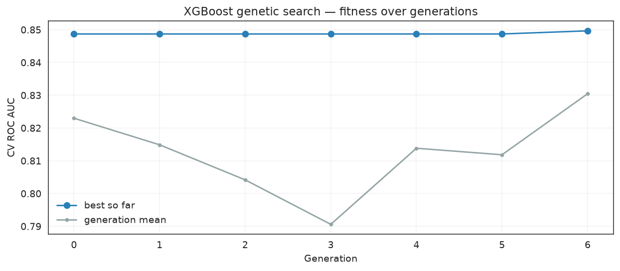
The interaction the search exploits
learning_rate and n_estimators trade off: more trees want a smaller step. Coloring every evaluated candidate by its CV score shows the productive region — a band of low learning rate with many estimators — that a one-parameter-at-a-time sweep would struggle to find.
results = pd.DataFrame(ga_search.cv_results_)
fig, ax = plt.subplots(figsize=(8, 5))
sc = ax.scatter(results["param_learning_rate"], results["param_n_estimators"],
                c=results["mean_test_score"], cmap="viridis", s=60, edgecolor="white")
ax.set_xscale("log")
ax.set_xlabel("learning_rate (log scale)")
ax.set_ylabel("n_estimators")
ax.set_title("Every evaluated candidate, colored by CV ROC AUC")
fig.colorbar(sc, label="mean CV ROC AUC")
fig.tight_layout()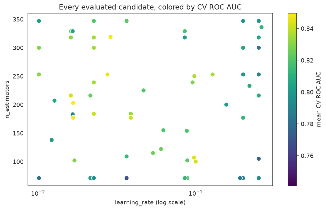
Feature importance of the tuned model
importances = pd.Series(ga_search.best_estimator_.feature_importances_,
                        index=[f"f{i:02d}" for i in range(X_train.shape[1])])
top = importances.sort_values(ascending=True).tail(15)
fig, ax = plt.subplots(figsize=(8, 6))
top.plot(kind="barh", ax=ax, color="#27ae60")
ax.set_title("Top-15 feature importances — tuned XGBoost")
ax.set_xlabel("importance (gain)")
fig.tight_layout()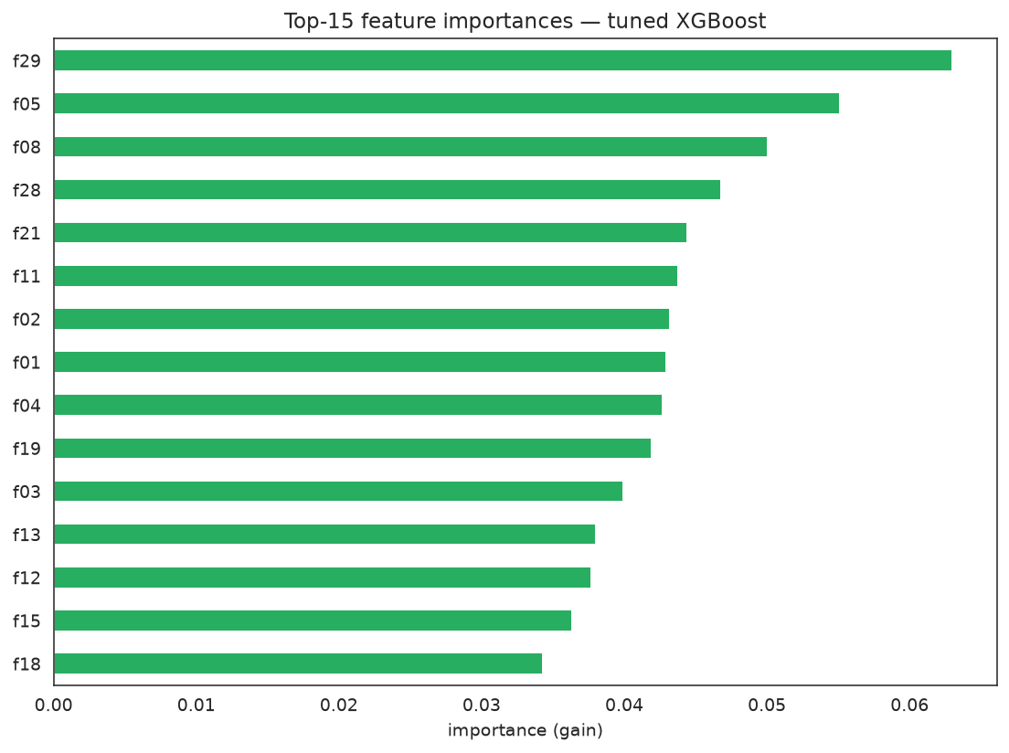
How Does It Compare to Random Search?
Random search is a strong baseline. Given the same evaluation budget and the same split, the genetic search is competitive while also returning per-generation telemetry and the diagnostic plots above. (On a small, smooth space the two will tie; the genetic search's edge grows with the number of interacting parameters.)
from scipy.stats import loguniform, randint, uniform
from sklearn.model_selection import RandomizedSearchCV

budget = ga_search.fit_stats_["unique_candidates"]
random_search = RandomizedSearchCV(
    XGBClassifier(tree_method="hist", eval_metric="logloss",
                  random_state=RANDOM_STATE, n_jobs=1),
    {
        "n_estimators": randint(50, 600), "max_depth": randint(2, 11),
        "min_child_weight": randint(1, 13), "subsample": uniform(0.5, 0.5),
        "colsample_bytree": uniform(0.4, 0.6), "learning_rate": loguniform(0.01, 0.3),
        "gamma": loguniform(1e-4, 1.0), "reg_alpha": loguniform(1e-5, 10.0),
        "reg_lambda": loguniform(1e-5, 10.0),
    },
    n_iter=budget, scoring="roc_auc", cv=cv, random_state=RANDOM_STATE, n_jobs=-1,
)
random_search.fit(X_train, y_train)
rnd_metrics = evaluate("RandomizedSearchCV", random_search)

table = pd.DataFrame([baseline_metrics, rnd_metrics, ga_metrics])
table["best_cv_auc"] = [None, round(random_search.best_score_, 4), round(ga_search.best_score_, 4)]
table["candidates"] = [None, budget, ga_search.fit_stats_["unique_candidates"]]
print(table.to_string(index=False)) model accuracy balanced_accuracy roc_auc best_cv_auc candidates
XGBoost defaults 0.794 0.7940 0.8608 NaN NaN
RandomizedSearchCV 0.805 0.8050 0.8861 0.8561 132.0
GASearchCV (tuned) 0.798 0.7979 0.8807 0.8497 132.0Practical Notes
tree_method="hist"dramatically cuts per-tree build time — use it by default.- Pair
n_jobs=1on any estimator that manages its own threads (XGBoost, LightGBM, CatBoost) withparallel_backend="cv"to avoid oversubscription. - Lower bounds in
warm_start_configsforlog-uniformparameters must be at the distribution's floor (e.g.1e-5), not0.0. - The headline win is tuning vs not tuning: the default booster overfits; the search finds a configuration that generalizes. Treat any random-search comparison as a tie-or-better sanity check, not the main event.
- Check
fit_stats_["cache_hits"]— non-zero means duplicate candidates from convergence are being recycled instead of recomputed.
See Also
- Tune LightGBM — leaf-wise trees and the
num_leaves/max_depthconstraint - Tune CatBoost — CatBoost-specific parameters
- Comparing Search Methods — GA vs random vs grid, honestly
- Advanced Optimizer Control — diversity, fitness sharing, local search