Development version

This is the latest (dev) documentation. It may contain unreleased features or breaking changes. For the stable release, use stable.

Pipeline Regression Tuning

This example tunes a scikit-learn Pipeline with GASearchCV. Pipeline parameters use the standard sklearn double-underscore syntax — regressor__max_depth reaches the max_depth of the step named regressor. We tune a StandardScaler + GradientBoostingRegressor pipeline on the diabetes dataset and measure the result the honest way: against a default, untuned model on an untouched test set.

Setup

We load the diabetes regression dataset (442 patients, 10 features) and hold out 30% for a final, untouched evaluation. Everything downstream is seeded for reproducibility.

import warnings
from pprint import pprint

import numpy as np
import pandas as pd
from sklearn.datasets import load_diabetes
from sklearn.ensemble import GradientBoostingRegressor
from sklearn.metrics import mean_absolute_error, mean_squared_error, r2_score
from sklearn.model_selection import KFold, train_test_split
from sklearn.pipeline import Pipeline
from sklearn.preprocessing import StandardScaler

from sklearn_genetic import (
    EvolutionConfig, GASearchCV, OptimizationConfig, PopulationConfig, RuntimeConfig,
)
from sklearn_genetic.callbacks import ConsecutiveStopping, DeltaThreshold, TimerStopping
from sklearn_genetic.schedules import ExponentialAdapter, InverseAdapter
from sklearn_genetic.space import Categorical, Continuous, Integer

warnings.filterwarnings("ignore")

RANDOM_STATE = 42

data = load_diabetes(as_frame=True)
X, y = data.data, data.target

X_train, X_test, y_train, y_test = train_test_split(
    X, y, test_size=0.30, random_state=RANDOM_STATE
)
cv = KFold(n_splits=4, shuffle=True, random_state=RANDOM_STATE)

print(f"Training shape: {X_train.shape}")
print(f"Test shape: {X_test.shape}")

Training shape: (309, 10)
Test shape: (133, 10)

Baseline Pipeline

Before tuning anything, fit a pipeline with default boosting settings. This is the number to beat — a model anyone gets for free with one line of code.

def make_pipeline(**regressor_kwargs):
    return Pipeline([
        ("scaler", StandardScaler()),
        ("regressor", GradientBoostingRegressor(random_state=RANDOM_STATE, **regressor_kwargs)),
    ])


def regression_metrics(estimator, X_eval, y_eval):
    predictions = estimator.predict(X_eval)
    rmse = mean_squared_error(y_eval, predictions) ** 0.5
    return {
        "r2": round(r2_score(y_eval, predictions), 4),
        "rmse": round(rmse, 2),
        "mae": round(mean_absolute_error(y_eval, predictions), 2),
    }


baseline = make_pipeline()
baseline.fit(X_train, y_train)
baseline_metrics = regression_metrics(baseline, X_test, y_test)
baseline_metrics

{'r2': 0.4303, 'rmse': 55.46, 'mae': 44.72}

Pipeline Search Space

Parameter names use the sklearn step__param convention, so every key below starts with regressor__ to target the boosting step inside the pipeline.

param_grid = {
    "regressor__n_estimators": Integer(40, 180),
    "regressor__learning_rate": Continuous(0.01, 0.20, distribution="log-uniform"),
    "regressor__max_depth": Integer(1, 4),
    "regressor__min_samples_leaf": Integer(1, 12),
    "regressor__subsample": Continuous(0.65, 1.0),
    "regressor__loss": Categorical(["squared_error", "absolute_error", "huber"]),
}
sorted(param_grid)

['regressor__learning_rate', 'regressor__loss', 'regressor__max_depth', 'regressor__min_samples_leaf', 'regressor__n_estimators', 'regressor__subsample']

Regression scorers

For metrics where smaller is better, use sklearn's negative scorer: "neg_root_mean_squared_error". The GA maximizes fitness, so negative RMSE increases (toward zero) exactly as RMSE decreases.

Configure GASearchCV

We keep the population and generations modest so the search finishes quickly, and warm-start it with a sensible hand-picked configuration so generation 0 already has a reasonable candidate to improve on.

search = GASearchCV(
    estimator=make_pipeline(),
    random_state=RANDOM_STATE,
    param_grid=param_grid,
    scoring="neg_root_mean_squared_error",
    criteria="max",
    cv=cv,
    evolution_config=EvolutionConfig(
        population_size=10,
        generations=8,
        crossover_probability=ExponentialAdapter(initial_value=0.8, end_value=0.4, adaptive_rate=0.15),
        mutation_probability=InverseAdapter(initial_value=0.25, end_value=0.08, adaptive_rate=0.25),
        tournament_size=3,
        elitism=True,
        keep_top_k=3,
    ),
    population_config=PopulationConfig(
        initializer="smart",
        warm_start_configs=[{
            "regressor__n_estimators": 100,
            "regressor__learning_rate": 0.05,
            "regressor__max_depth": 2,
            "regressor__min_samples_leaf": 4,
            "regressor__subsample": 0.85,
            "regressor__loss": "squared_error",
        }],
    ),
    runtime_config=RuntimeConfig(
        n_jobs=-1,
        parallel_backend="auto",
        use_cache=True,
        verbose=False,
        return_train_score=False,
    ),
    optimization_config=OptimizationConfig(
        local_search=True,
        local_search_top_k=2,
        local_search_steps=1,
        local_search_radius=0.20,
        diversity_control=True,
        diversity_threshold=0.30,
        diversity_stagnation_generations=3,
        diversity_mutation_boost=1.8,
        random_immigrants_fraction=0.10,
        fitness_sharing=True,
        sharing_radius=0.40,
    ),
)

callbacks = [
    DeltaThreshold(threshold=0.01, generations=5, metric="fitness_best"),
    ConsecutiveStopping(generations=7, metric="fitness_best"),
    TimerStopping(total_seconds=75),
]

search.fit(X_train, y_train, callbacks=callbacks)
print("fitted:", search.best_score_ is not None)

INFO: TimerStopping callback met its criteria
INFO: Stopping the algorithm
fitted: True

Evaluate Predictions

GASearchCV refits the best pipeline automatically, so you can call predict directly on the search object. The holdout comparison is the fastest sanity check: the GA should earn its extra search cost by improving the metrics you actually care about outside cross-validation.

print("Best CV negative RMSE:", round(search.best_score_, 4))
print("Best params:")
pprint(search.best_params_)

ga_metrics = regression_metrics(search, X_test, y_test)
comparison = pd.DataFrame(
    [baseline_metrics, ga_metrics],
    index=["default GBR", "GA-tuned pipeline"],
)
comparison

Best CV negative RMSE: -58.5933
Best params:
{'regressor__learning_rate': 0.05,
 'regressor__loss': 'squared_error',
 'regressor__max_depth': 1,
 'regressor__min_samples_leaf': 9,
 'regressor__n_estimators': 119,
 'regressor__subsample': 0.7807245051751381}
                       r2   rmse    mae
default GBR        0.4303  55.46  44.72
GA-tuned pipeline  0.4987  52.02  41.77

r2_gain = ga_metrics["r2"] - baseline_metrics["r2"]
rmse_drop = baseline_metrics["rmse"] - ga_metrics["rmse"]
mae_drop = baseline_metrics["mae"] - ga_metrics["mae"]
print(f"R2  : {baseline_metrics['r2']:.4f}  ->  {ga_metrics['r2']:.4f}   ({r2_gain:+.4f})")
print(f"RMSE: {baseline_metrics['rmse']:.2f}  ->  {ga_metrics['rmse']:.2f}   ({-rmse_drop:+.2f})")
print(f"MAE : {baseline_metrics['mae']:.2f}  ->  {ga_metrics['mae']:.2f}   ({-mae_drop:+.2f})")

R2  : 0.4303  ->  0.4987   (+0.0684)
RMSE: 55.46  ->  52.02   (-3.44)
MAE : 44.72  ->  41.77   (-2.95)

Plotting the same numbers makes the improvement on every metric obvious at a glance.

import matplotlib.pyplot as plt

labels = ["R2", "RMSE", "MAE"]
base_vals = [baseline_metrics["r2"], baseline_metrics["rmse"], baseline_metrics["mae"]]
ga_vals = [ga_metrics["r2"], ga_metrics["rmse"], ga_metrics["mae"]]

fig, axes = plt.subplots(1, 3, figsize=(11, 3.6))
colors = ["#95a5a6", "#16a085"]
for ax, label, b, g in zip(axes, labels, base_vals, ga_vals):
    bars = ax.bar(["default", "GA-tuned"], [b, g], color=colors, width=0.6)
    ax.set_title(label)
    ax.bar_label(bars, fmt="%.3g", padding=3)
    ax.margins(y=0.18)
    ax.grid(axis="y", alpha=0.25)
axes[0].set_ylabel("score")
fig.suptitle("Default GradientBoostingRegressor vs GA-tuned pipeline (holdout)")
fig.tight_layout()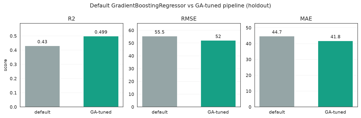

Higher R2 and lower RMSE/MAE for the GA-tuned pipeline — tuning beats the defaults on every metric.

Search Cost and Telemetry

fit_stats_ reports the evaluation accounting (how many candidates were actually scored, cache hits, random immigrants, local refinements), and history carries the per-generation convergence and diversity signals.

print(search.fit_stats_)

{'evaluated_candidates': 72, 'unique_candidates': 72, 'cross_validate_calls': 72, 'cache_hits': 0, 'duplicate_candidates': 0, 'skipped_invalid_candidates': 0, 'population_parallel_batches': 5, 'population_serial_batches': 0, 'random_immigrants': 0, 'local_refinement_candidates': 2}

history = pd.DataFrame(search.history)
cols = ["gen", "fitness", "fitness_max", "unique_individual_ratio",
        "genotype_diversity", "stagnation_generations"]
history[[c for c in cols if c in history.columns]].tail()

   gen    fitness  fitness_max  unique_individual_ratio  genotype_diversity  stagnation_generations
0    0 -61.243523   -59.037963                      1.0            0.722222                       0
1    1 -59.857250   -59.037963                      0.8            0.407407                       1
2    2 -60.193052   -59.045795                      0.6            0.388889                       2
3    3 -59.580004   -58.664782                      0.7            0.351852                       0

Visualize the Search

A fitted search can answer more pointed questions than "what won?". This landscape colors each evaluated candidate by its CV score across a learning-rate / tree-depth slice, highlighting which region was consistently promising.

from sklearn_genetic.plots import plot_cv_scores, plot_score_landscape

plot_score_landscape(
    search,
    x="regressor__learning_rate",
    y="regressor__max_depth",
)
plt.tight_layout()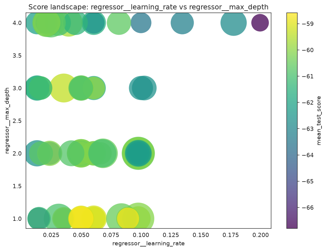

Each point is one evaluated candidate; brighter points scored better in cross-validation.

When several candidates have similar mean scores, inspect fold-level stability before trusting a tiny ranking difference.

plot_cv_scores(
    search,
    top_k=5,
    label_params=["regressor__learning_rate", "regressor__max_depth"],
)
plt.tight_layout()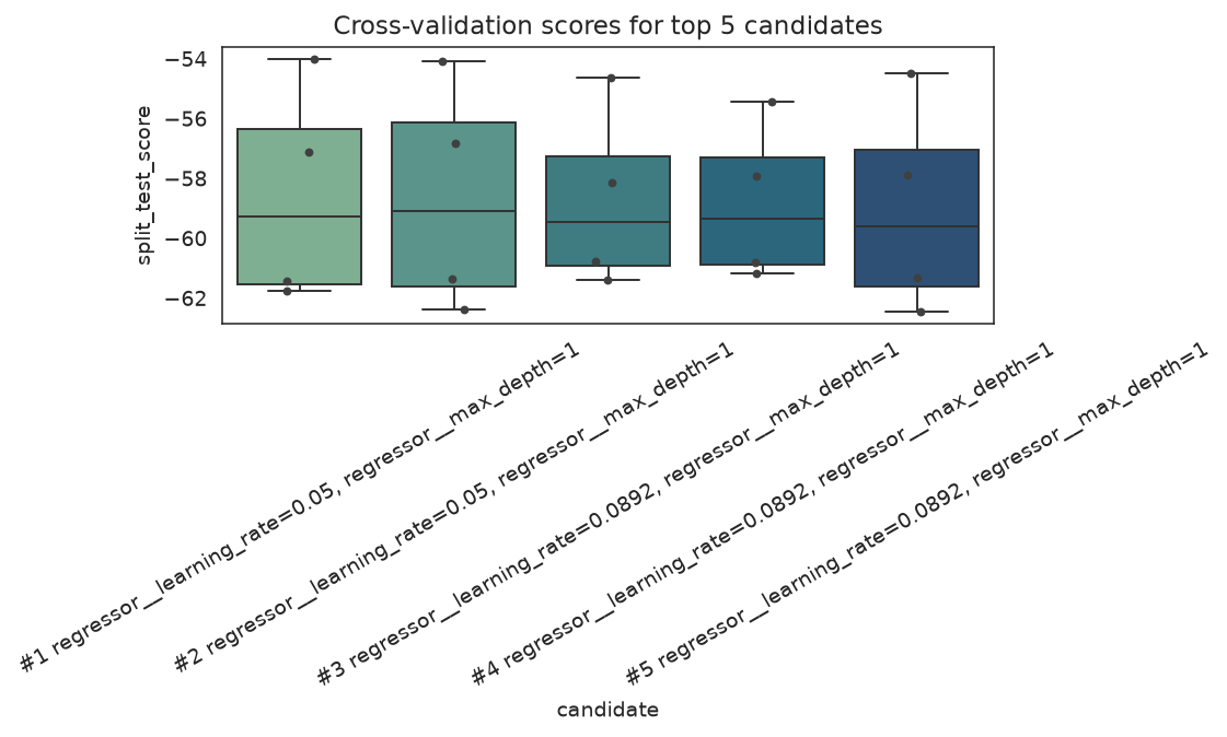

Per-fold spread for the strongest candidates — a narrow box means a stable choice.

Practical Notes

• Use pipeline parameter names exactly as sklearn expects them (step__param).
• For regression losses where smaller is better, use sklearn's negative scorers such as "neg_root_mean_squared_error"; the GA maximizes fitness.
• Compare holdout metrics, not only CV fitness — the default model is the honest baseline to beat.
• If the search revisits many candidates, inspect cache_hits in fit_stats_ and consider stronger diversity controls or a wider search space.

See Also

• Pipeline Tuning Guide — pipeline parameter naming and step configuration
• Search Space API — Continuous, Integer, Categorical reference
• Plots API — convergence, landscape, CV stability, and candidate-ranking plots