Multi-Metric Search on Imbalanced Data

Multi-metric search shines when your metrics disagree. On a balanced, easy dataset, accuracy, balanced accuracy, and F1 all crown the same candidate and there is nothing to choose between them. So we use a deliberately imbalanced problem — 90% of one class, 10% of the other — where a model can look great on accuracy while quietly ignoring the minority class. Here refit is a real decision, and the per-metric cv_results_ actually rank candidates differently.

Setup

We build a 2,000-sample binary problem with a 90/10 class split and a bit of label noise. The majority class is so dominant that a model predicting "always majority" already scores 90% accuracy — which is exactly why accuracy alone is misleading here.

import warnings
from pprint import pprint

import numpy as np
import pandas as pd
from sklearn.datasets import make_classification
from sklearn.linear_model import LogisticRegression
from sklearn.metrics import accuracy_score, balanced_accuracy_score, f1_score, make_scorer
from sklearn.model_selection import StratifiedKFold, train_test_split
from sklearn.pipeline import Pipeline
from sklearn.preprocessing import StandardScaler

from sklearn_genetic import (
    EvolutionConfig, GASearchCV, OptimizationConfig, PopulationConfig, RuntimeConfig,
)
from sklearn_genetic.callbacks import ConsecutiveStopping, DeltaThreshold, TimerStopping
from sklearn_genetic.plots import plot_candidate_rankings
from sklearn_genetic.schedules import ExponentialAdapter, InverseAdapter
from sklearn_genetic.space import Categorical, Continuous, Integer

warnings.filterwarnings("ignore")

RANDOM_STATE = 42

X, y = make_classification(
    n_samples=2000,
    n_features=20,
    n_informative=8,
    weights=[0.9, 0.1],
    flip_y=0.03,
    random_state=RANDOM_STATE,
)
X = pd.DataFrame(X, columns=[f"f{i:02d}" for i in range(X.shape[1])])

X_train, X_test, y_train, y_test = train_test_split(
    X, y, test_size=0.30, stratify=y, random_state=RANDOM_STATE
)
cv = StratifiedKFold(n_splits=3, shuffle=True, random_state=RANDOM_STATE)

counts = np.bincount(y)
print(f"class balance: {counts[0]} majority / {counts[1]} minority "
      f"({counts[1] / counts.sum():.0%} minority)")
print(f"train={X_train.shape}  test={X_test.shape}")

class balance: 1776 majority / 224 minority (11% minority)
train=(1400, 20)  test=(600, 20)

Define Multiple Metrics

A multi-metric search receives a dictionary of scorers. On this dataset the three metrics measure very different things:

• accuracy — fraction correct; flattered by the dominant majority class.
• balanced_accuracy — average recall across classes; punishes ignoring the minority.
• f1 — harmonic mean of precision and recall on the minority class.

The refit parameter decides which metric chooses best_params_ and refits best_estimator_. We refit on balanced_accuracy so the final model is forced to take the minority class seriously.

scoring = {
    "accuracy": "accuracy",
    "balanced_accuracy": make_scorer(balanced_accuracy_score),
    "f1": make_scorer(f1_score),  # minority (positive) class F1
}
sorted(scoring)

['accuracy', 'balanced_accuracy', 'f1']

Configure GASearchCV

We tune a scaled LogisticRegression. The key knob for imbalance is class_weight: leaving it None chases accuracy, while "balanced" reweights the minority class — so different candidates will favor different metrics, exactly the tension we want to expose.

model = Pipeline([
    ("scaler", StandardScaler()),
    ("logistic", LogisticRegression(solver="saga", max_iter=1500, random_state=RANDOM_STATE)),
])

param_grid = {
    "logistic__C": Continuous(1e-3, 30.0, distribution="log-uniform"),
    "logistic__l1_ratio": Continuous(0.0, 1.0),
    "logistic__class_weight": Categorical([None, "balanced"]),
    "logistic__max_iter": Integer(1200, 1800),
}

search = GASearchCV(
    estimator=model,
    random_state=RANDOM_STATE,
    param_grid=param_grid,
    scoring=scoring,
    refit="balanced_accuracy",   # drives best_params_ and best_estimator_
    cv=cv,
    evolution_config=EvolutionConfig(
        population_size=12,
        generations=10,
        crossover_probability=ExponentialAdapter(initial_value=0.8, end_value=0.4, adaptive_rate=0.15),
        mutation_probability=InverseAdapter(initial_value=0.25, end_value=0.08, adaptive_rate=0.25),
        tournament_size=3,
        elitism=True,
        keep_top_k=3,
    ),
    population_config=PopulationConfig(
        initializer="smart",
        warm_start_configs=[{
            "logistic__C": 1.0,
            "logistic__l1_ratio": 0.0,
            "logistic__class_weight": None,
            "logistic__max_iter": 1300,
        }],
    ),
    runtime_config=RuntimeConfig(n_jobs=-1, parallel_backend="auto", use_cache=True, verbose=False),
    optimization_config=OptimizationConfig(
        local_search=True,
        local_search_top_k=2,
        local_search_steps=1,
        local_search_radius=0.20,
        diversity_control=True,
        diversity_threshold=0.30,
        diversity_stagnation_generations=3,
        diversity_mutation_boost=1.8,
        random_immigrants_fraction=0.10,
        fitness_sharing=True,
        sharing_radius=0.40,
    ),
)

callbacks = [
    DeltaThreshold(threshold=0.001, generations=5, metric="fitness_best"),
    ConsecutiveStopping(generations=7, metric="fitness_best"),
    TimerStopping(total_seconds=90),
]

search.fit(X_train, y_train, callbacks=callbacks)
print("fitted:", search.refit_metric)

INFO: DeltaThreshold callback met its criteria
INFO: Stopping the algorithm
fitted: balanced_accuracy

Best Parameters and Test Metrics

Because refit="balanced_accuracy", best_params_ and best_estimator_ are selected by the CV rank of that metric.

print("Refit metric:", search.refit_metric)
print("Best balanced-accuracy CV score:", round(search.best_score_, 4))
print("Best params:")
pprint(search.best_params_)

predictions = search.predict(X_test)
test_metrics = {
    "accuracy": round(accuracy_score(y_test, predictions), 4),
    "balanced_accuracy": round(balanced_accuracy_score(y_test, predictions), 4),
    "f1": round(f1_score(y_test, predictions), 4),
}
test_metrics

Refit metric: balanced_accuracy
Best balanced-accuracy CV score: 0.7046
Best params:
{'logistic__C': 0.040979535386389716,
 'logistic__class_weight': 'balanced',
 'logistic__l1_ratio': 0.9046094635389027,
 'logistic__max_iter': 1799}
{'accuracy': 0.73, 'balanced_accuracy': 0.698, 'f1': 0.352}

Explore Multi-Metric cv_results_

For multi-metric searches, cv_results_ contains one set of columns per metric. The point of this page is visible right here: sorting by each metric's rank surfaces a different top candidate.

results = pd.DataFrame(search.cv_results_)
metric_columns = [
    "mean_test_accuracy", "rank_test_accuracy",
    "mean_test_balanced_accuracy", "rank_test_balanced_accuracy",
    "mean_test_f1", "rank_test_f1",
]
param_columns = ["param_logistic__C", "param_logistic__class_weight"]

results[metric_columns + param_columns].sort_values("rank_test_balanced_accuracy").head()

     mean_test_accuracy  rank_test_accuracy  mean_test_balanced_accuracy  rank_test_balanced_accuracy  mean_test_f1  rank_test_f1  param_logistic__C param_logistic__class_weight
97             0.712123                  60                     0.704607                            1      0.351874             1           0.040980                     balanced
33             0.707845                  66                     0.702020                            2      0.347684             6           2.735191                     balanced
109            0.707845                  66                     0.702020                            2      0.347684             6           2.735191                     balanced
58             0.707130                  69                     0.701617                            4      0.347158             8          11.585019                     balanced
43             0.711408                  62                     0.701400                            5      0.349366             2           0.044433                     balanced

The Metrics Disagree

The same cv_results_ can point to different winners. Pulling the best row for each metric — without rerunning the search — shows the tradeoff explicitly: accuracy tends to prefer the unweighted model, while balanced accuracy and F1 reward the candidate that pays attention to the minority class.

best_rows = []
for metric_name in ["accuracy", "balanced_accuracy", "f1"]:
    row = results.sort_values(f"rank_test_{metric_name}").iloc[0]
    best_rows.append({
        "winning_metric": metric_name,
        "candidate_index": int(row.name),
        "accuracy": round(row["mean_test_accuracy"], 4),
        "balanced_accuracy": round(row["mean_test_balanced_accuracy"], 4),
        "f1": round(row["mean_test_f1"], 4),
        "class_weight": row["param_logistic__class_weight"],
        "C": round(float(row["param_logistic__C"]), 3),
    })

pd.DataFrame(best_rows)

      winning_metric  candidate_index  accuracy  balanced_accuracy      f1 class_weight      C
0           accuracy               75    0.8957             0.5630  0.2215         None  1.650
1  balanced_accuracy               97    0.7121             0.7046  0.3519     balanced  0.041
2                 f1               97    0.7121             0.7046  0.3519     balanced  0.041

winners = {
    m: int(results.sort_values(f"rank_test_{m}").iloc[0].name)
    for m in ["accuracy", "balanced_accuracy", "f1"]
}
distinct = len(set(winners.values()))
print("top candidate index per metric:", winners)
print(f"{distinct} distinct candidates win across the 3 metrics "
      f"-> the metrics disagree." if distinct > 1
      else "metrics agreed on a single candidate.")

top candidate index per metric: {'accuracy': 75, 'balanced_accuracy': 97, 'f1': 97}
2 distinct candidates win across the 3 metrics -> the metrics disagree.

For advanced users the useful question is not only "which candidate won?", but whether different metrics prefer the same region. Plotting the top candidates per metric makes those tradeoffs visible without rerunning the search.

import matplotlib.pyplot as plt

fig, axes = plt.subplots(1, 3, figsize=(15, 4))
for axis, metric in zip(axes, ["accuracy", "balanced_accuracy", "f1"]):
    plot_candidate_rankings(
        search,
        top_k=6,
        metric=metric,
        label_params=["logistic__C", "logistic__class_weight"],
        ax=axis,
        title=metric,
    )
fig.suptitle("Top candidates by metric — each metric prefers a different ordering")
fig.tight_layout()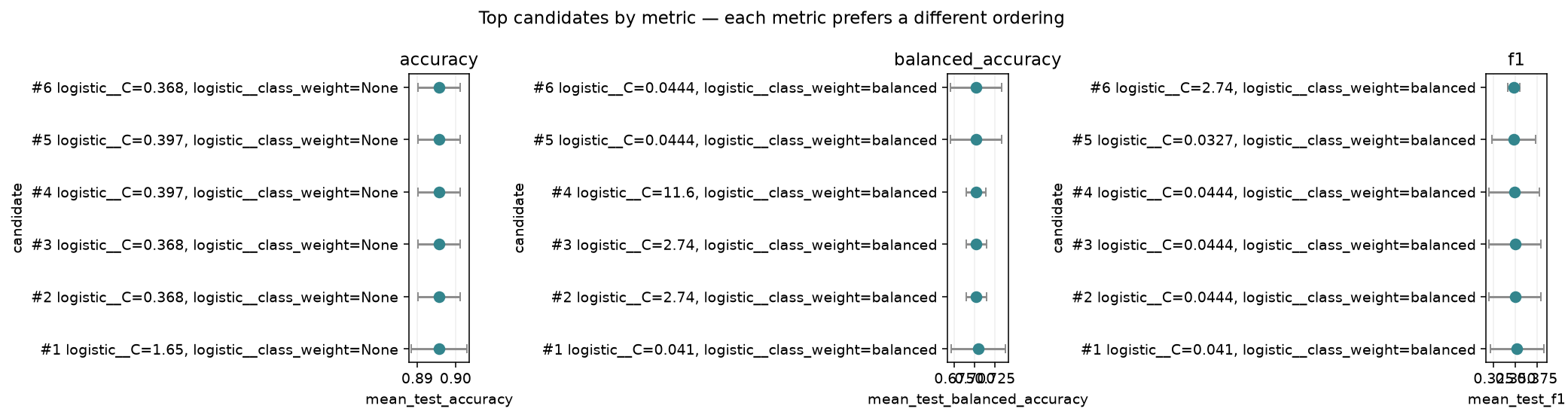

Each subplot ranks candidates by one metric; the orderings differ, so the refit choice matters.

Optimizer Telemetry

With multi-metric scoring the GA still optimizes a single scalar fitness — the selected refit metric. Telemetry explains how the optimizer moved through the space while optimizing balanced accuracy.

print(search.fit_stats_)

{'evaluated_candidates': 110, 'unique_candidates': 110, 'cross_validate_calls': 110, 'cache_hits': 0, 'duplicate_candidates': 0, 'skipped_invalid_candidates': 0, 'population_parallel_batches': 6, 'population_serial_batches': 0, 'random_immigrants': 0, 'local_refinement_candidates': 2}

history = pd.DataFrame(search.history)
cols = ["gen", "fitness", "fitness_max", "fitness_std",
        "unique_individual_ratio", "genotype_diversity", "stagnation_generations"]
history[[c for c in cols if c in history.columns]].tail()

   gen   fitness  fitness_max  fitness_std  unique_individual_ratio  genotype_diversity  stagnation_generations
0    0  0.591005     0.701215     0.078317                 1.000000            0.727273                       0
1    1  0.654288     0.701215     0.078101                 0.750000            0.431818                       1
2    2  0.578690     0.701400     0.073626                 0.666667            0.454545                       0
3    3  0.676753     0.701400     0.051773                 0.583333            0.431818                       1
4    4  0.644290     0.702020     0.066832                 0.583333            0.340909                       0

Practical Notes

• Set refit to the metric that should define the final model before fitting; on imbalanced data, accuracy is rarely the right choice.
• best_score_, best_params_, and best_estimator_ follow the refit metric, not every metric at once.
• Use cv_results_ to inspect tradeoffs between metrics after fitting — when the ranks disagree, you are seeing a genuine modeling decision.
• Use fit_stats_ and history to understand optimizer cost, diversity, stagnation, and convergence.

See Also

• Multi-Metric Optimization Guide — full guide with scoring dict details
• GASearchCV API — scoring and refit parameter reference
• Understanding Cross-Validation — reading the generation log