Comprehensive GA Feature Selection

Choosing which of n columns to keep is a search over 2ⁿ subsets — far beyond any grid or random sweep. GAFeatureSelectionCV evolves the on/off mask directly, and because it scores whole subsets it can account for redundancy and interaction between columns, not just each column in isolation.

This tutorial is a full multi-stage walkthrough. We build a dataset whose informative, redundant, and pure-noise columns are known, then show the genetic search decisively beating the all-features baseline on a held-out test set. We grade the mask against the ground truth, confirm the win transfers to a completely different estimator, and read the convergence and support telemetry.

Prerequisites

• sklearn-genetic-opt installed (pip install sklearn-genetic-opt).
• For the plots, the seaborn extra: pip install sklearn-genetic-opt[all].
• Comfort with scikit-learn pipelines and cross-validation.

Stage 1 — A Dataset With Known Signal

We generate 1,500 samples with 60 features, of which only the first 20 carry information (12 informative + 8 redundant linear combinations). The remaining 40 columns are pure noise. shuffle=False keeps the columns in that order so we can grade the selection against the truth later.

import warnings
import numpy as np
import pandas as pd
from sklearn.datasets import make_classification
from sklearn.metrics import accuracy_score, balanced_accuracy_score
from sklearn.model_selection import StratifiedKFold, cross_val_score, train_test_split
from sklearn.neighbors import KNeighborsClassifier
from sklearn.pipeline import Pipeline
from sklearn.preprocessing import StandardScaler
from sklearn.svm import SVC

from sklearn_genetic import (
    EvolutionConfig,
    GAFeatureSelectionCV,
    OptimizationConfig,
    PopulationConfig,
    RuntimeConfig,
)
from sklearn_genetic.callbacks import ConsecutiveStopping, DeltaThreshold

warnings.filterwarnings("ignore")
RANDOM_STATE = 42

N_INFORMATIVE, N_REDUNDANT, N_NOISE = 12, 8, 40
n_features = N_INFORMATIVE + N_REDUNDANT + N_NOISE  # 60

X_array, y = make_classification(
    n_samples=1500,
    n_features=n_features,
    n_informative=N_INFORMATIVE,
    n_redundant=N_REDUNDANT,
    n_repeated=0,
    n_clusters_per_class=2,
    class_sep=0.8,
    flip_y=0.02,
    shuffle=False,            # keep informative / redundant / noise columns in order
    random_state=RANDOM_STATE,
)

feature_names = (
    [f"info_{i:02d}" for i in range(N_INFORMATIVE)]
    + [f"redundant_{i:02d}" for i in range(N_REDUNDANT)]
    + [f"noise_{i:02d}" for i in range(N_NOISE)]
)
is_signal = np.array([not name.startswith("noise") for name in feature_names])
X = pd.DataFrame(X_array, columns=feature_names)

X_train, X_test, y_train, y_test = train_test_split(
    X, y, test_size=0.40, stratify=y, random_state=RANDOM_STATE
)
cv = StratifiedKFold(n_splits=3, shuffle=True, random_state=RANDOM_STATE)
print(f"{n_features} features: {is_signal.sum()} carry signal, {(~is_signal).sum()} are noise")
print(f"train={X_train.shape}  test={X_test.shape}")

60 features: 20 carry signal, 40 are noise
train=(900, 60)  test=(600, 60)

Stage 2 — Why This Model Needs Feature Selection

We use a k-nearest-neighbours classifier. Distance-based models are the textbook victim of the curse of dimensionality: 40 irrelevant columns drown the distance metric, so every prediction is made in a fog of noise. That makes this a problem where keeping the right columns is worth real accuracy.

We also keep a second, completely different estimator on hand — an SVC with an RBF kernel, also distance/kernel based. If the GA's selection is genuine signal rather than an artefact of the KNN scorer, the SVC should benefit from the same subset.

def make_knn():
    return Pipeline([
        ("scaler", StandardScaler()),
        ("knn", KNeighborsClassifier(n_neighbors=15)),
    ])


def make_svc():
    return Pipeline([
        ("scaler", StandardScaler()),
        ("svc", SVC(kernel="rbf", C=2.0, gamma="scale", random_state=RANDOM_STATE)),
    ])


def holdout_scores(make_model, columns=None):
    Xtr = X_train if columns is None else X_train.iloc[:, columns]
    Xte = X_test if columns is None else X_test.iloc[:, columns]
    model = make_model().fit(Xtr, y_train)
    pred = model.predict(Xte)
    return {
        "accuracy": round(accuracy_score(y_test, pred), 4),
        "balanced_accuracy": round(balanced_accuracy_score(y_test, pred), 4),
    }


knn_all_cv = cross_val_score(
    make_knn(), X_train, y_train, cv=cv, scoring="balanced_accuracy"
).mean()
knn_all = holdout_scores(make_knn)
svc_all = holdout_scores(make_svc)

print(f"KNN, all {n_features} features : CV bal-acc = {knn_all_cv:.4f}, "
      f"holdout bal-acc = {knn_all['balanced_accuracy']:.4f}")
print(f"SVC, all {n_features} features : holdout bal-acc = {svc_all['balanced_accuracy']:.4f}")

KNN, all 60 features : CV bal-acc = 0.7625, holdout bal-acc = 0.8001
SVC, all 60 features : holdout bal-acc = 0.8633

Stage 3 — Evolve the Feature Mask

GAFeatureSelectionCV searches over binary masks — 1 keeps a column, 0 drops it. We optimize cross-validated balanced accuracy of the KNN model, with the advanced controls switched on:

• smart initialization for broad first-generation coverage,
• a steady mutation rate that keeps probing column flips throughout the run,
• diversity control + fitness sharing so the population does not collapse onto one mask,
• local search for a final refinement pass onto a compact subset.

selector = GAFeatureSelectionCV(
    estimator=make_knn(),
    random_state=RANDOM_STATE,
    cv=cv,
    scoring="balanced_accuracy",
    evolution_config=EvolutionConfig(
        population_size=24,
        generations=20,
        crossover_probability=0.8,
        mutation_probability=0.12,
        tournament_size=3,
        elitism=True,
        keep_top_k=3,
    ),
    population_config=PopulationConfig(initializer="smart"),
    runtime_config=RuntimeConfig(n_jobs=-1, use_cache=True, verbose=False),
    optimization_config=OptimizationConfig(
        diversity_control=True,
        fitness_sharing=True,
        local_search=True,
        local_search_top_k=2,
    ),
)

callbacks = [
    DeltaThreshold(threshold=0.0005, generations=6, metric="fitness_best"),
    ConsecutiveStopping(generations=8, metric="fitness_best"),
]
selector.fit(X_train, y_train, callbacks=callbacks)

ga_best_cv = float(pd.DataFrame(selector.history)["fitness_best"].max())
print(f"Best CV balanced accuracy: {ga_best_cv:.4f}")
print(f"Selected {int(selector.support_.sum())} of {n_features} features")

Best CV balanced accuracy: 0.8024
Selected 32 of 60 features

Stage 4 — Grade the Mask Against the Truth

Because we know which columns are real, we can grade the selection directly: how much signal did it keep, and how much noise did it correctly throw away?

support = selector.support_
selected_idx = np.where(support)[0]
n_selected = int(support.sum())

print(f"Selected {n_selected} of {n_features} features")
print(f"  signal kept   : {int(is_signal[support].sum())} / {int(is_signal.sum())}")
print(f"  noise dropped : {int((~is_signal & ~support).sum())} / {int((~is_signal).sum())}")
print(f"  noise leaked  : {int((~is_signal[support]).sum())}")

Selected 32 of 60 features
  signal kept   : 17 / 20
  noise dropped : 25 / 40
  noise leaked  : 15

The support mask

import matplotlib.pyplot as plt
from sklearn_genetic.plots import plot_feature_selection

plot_feature_selection(selector, feature_names=feature_names)
fig = plt.gcf()
fig.set_size_inches(11, 9)
plt.title("Selected feature mask  (info | redundant | noise, top to bottom)")
plt.tight_layout()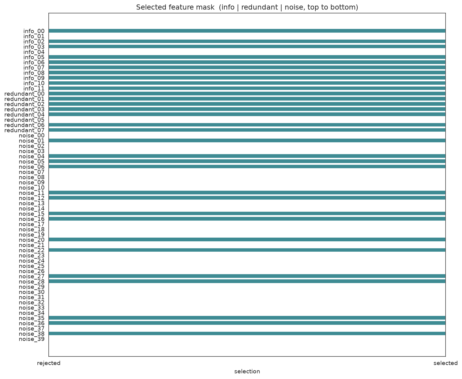

The search concentrates its picks in the info/redundant block and clears most of the noise block.

Fitness over generations

from sklearn_genetic.plots import plot_fitness_evolution

ax = plot_fitness_evolution(
    selector,
    metrics=["fitness_best", "fitness"],
    title="CV balanced accuracy climbs as noisy columns are pruned",
)
ax.set_xlabel("generation")
ax.figure.set_size_inches(8, 4.5)
ax.figure.tight_layout()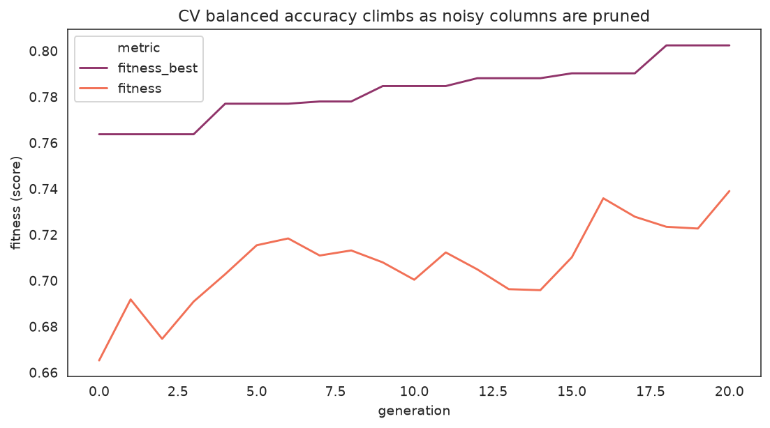

Best-so-far fitness rises as the search prunes noise columns; the population mean trails the leading edge.

Stage 5 — The Verdict (KNN)

Both rows use the same KNN model and the same split — the only difference is which columns reach it.

knn_sel = holdout_scores(make_knn, selected_idx)

verdict = pd.DataFrame([
    {"strategy": "All 60 features", "n_features": n_features,
     "cv_balanced_acc": round(knn_all_cv, 4), **knn_all},
    {"strategy": "GA-selected subset", "n_features": n_selected,
     "cv_balanced_acc": round(ga_best_cv, 4), **knn_sel},
])
print(verdict.to_string(index=False))
print()
gain = knn_sel["balanced_accuracy"] - knn_all["balanced_accuracy"]
print(f"Genetic feature selection lifts KNN holdout balanced accuracy by {gain:+.4f}")
print(f"while using only {n_selected} of {n_features} columns "
      f"({n_selected / n_features:.0%} of the inputs).")

          strategy  n_features  cv_balanced_acc  accuracy  balanced_accuracy
   All 60 features          60           0.7625     0.800             0.8001
GA-selected subset          32           0.8024     0.835             0.8350

Genetic feature selection lifts KNN holdout balanced accuracy by +0.0349
while using only 32 of 60 columns (53% of the inputs).

Stage 6 — Does the Win Transfer? (SVC robustness check)

The mask was selected to please the KNN scorer. The honest test of whether it found real signal is to hand the same subset to a completely different model. If an independent SVC-RBF also improves, the selection is model-agnostic signal, not a KNN-specific artefact.

svc_sel = holdout_scores(make_svc, selected_idx)

transfer = pd.DataFrame([
    {"model": "KNN", "all_features": knn_all["balanced_accuracy"],
     "selected": knn_sel["balanced_accuracy"],
     "delta": round(knn_sel["balanced_accuracy"] - knn_all["balanced_accuracy"], 4)},
    {"model": "SVC-RBF", "all_features": svc_all["balanced_accuracy"],
     "selected": svc_sel["balanced_accuracy"],
     "delta": round(svc_sel["balanced_accuracy"] - svc_all["balanced_accuracy"], 4)},
])
print(transfer.to_string(index=False))

  model  all_features  selected  delta
    KNN        0.8001    0.8350 0.0349
SVC-RBF        0.8633    0.8733 0.0100

Before / after feature-count and accuracy

fig, (ax_count, ax_acc) = plt.subplots(1, 2, figsize=(11, 4.5))

ax_count.bar(["all features", "GA-selected"], [n_features, n_selected],
             color=["#bdc3c7", "#16a085"])
ax_count.set_ylabel("number of features")
ax_count.set_title("Feature count")
for i, v in enumerate([n_features, n_selected]):
    ax_count.text(i, v + 0.5, str(v), ha="center")

labels = ["KNN", "SVC-RBF"]
all_vals = [knn_all["balanced_accuracy"], svc_all["balanced_accuracy"]]
sel_vals = [knn_sel["balanced_accuracy"], svc_sel["balanced_accuracy"]]
xpos = np.arange(len(labels))
width = 0.38
ax_acc.bar(xpos - width / 2, all_vals, width, label="all features", color="#bdc3c7")
ax_acc.bar(xpos + width / 2, sel_vals, width, label="GA-selected", color="#16a085")
ax_acc.set_xticks(xpos, labels)
ax_acc.set_ylabel("holdout balanced accuracy")
ax_acc.set_ylim(min(all_vals + sel_vals) - 0.05, max(all_vals + sel_vals) + 0.03)
ax_acc.set_title("Accuracy: all features vs GA-selected")
ax_acc.legend(frameon=False)
fig.tight_layout()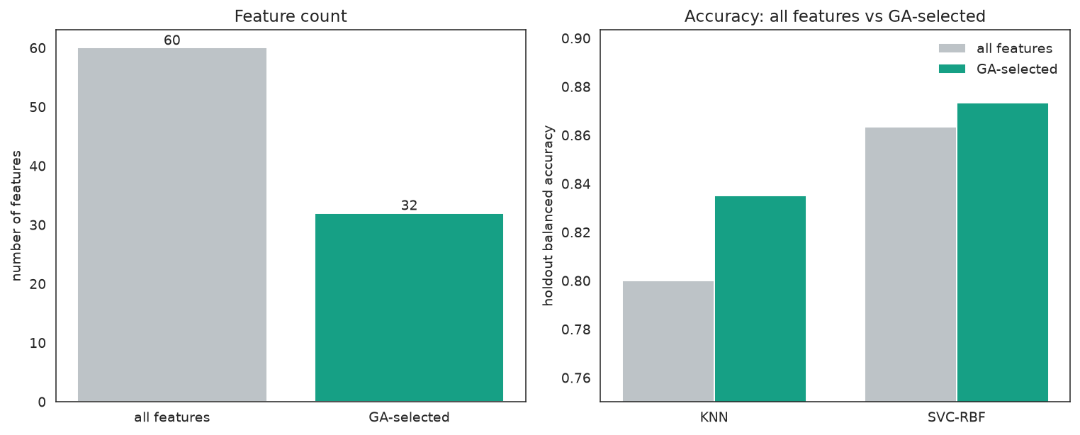

Left: the GA keeps a fraction of the columns. Right: both the KNN scorer and the independent SVC improve on the GA-selected subset.

Both estimators improve on the GA-selected subset even though only the KNN guided the search — the selected columns are genuine, model-agnostic signal.

Telemetry

fit_stats_ reports the evaluation accounting; history carries the per-generation convergence and diversity signals.

print(pd.Series(selector.fit_stats_).to_string())

evaluated_candidates           986
unique_candidates              986
cross_validate_calls           986
cache_hits                       0
duplicate_candidates             0
skipped_invalid_candidates       0
population_parallel_batches     22
population_serial_batches        0
random_immigrants              100
local_refinement_candidates      2

history = pd.DataFrame(selector.history)
cols = ["gen", "fitness", "fitness_best", "genotype_diversity",
        "unique_individual_ratio", "stagnation_generations"]
history[[c for c in cols if c in history.columns]].tail()

    gen   fitness  fitness_best  genotype_diversity  unique_individual_ratio  stagnation_generations
16   16  0.735777      0.790190            0.043478                 0.750000                       1
17   17  0.727760      0.790190            0.043478                 0.791667                       2
18   18  0.723373      0.802352            0.043478                 0.875000                       0
19   19  0.722615      0.802352            0.043478                 0.875000                       1
20   20  0.738935      0.802352            0.042754                 0.750000                       3

Practical Notes

• Pass max_features=k to force compact subsets when inference cost or interpretability matters; selector.support_.sum() is the actual count.
• Always compare against the all-features baseline — a smaller subset is only worth it if quality holds or improves.
• Cross-estimator validation (Stage 6) is the most reliable check that the selection is signal and not scorer-specific. If only the scoring estimator improves, suspect feature/scorer circularity.
• Feature selection helps most for models hurt by irrelevant inputs (distance- and kernel-based methods like KNN and SVC-RBF); strongly regularized linear models are already robust to noise columns.
• use_cache=True is especially impactful here — many masks differ by a single column, so cached evaluations avoid redundant CV calls.
• If diversity collapses early, lean on diversity_control, random_immigrants_fraction, and fitness_sharing before adding generations.

Next Steps

• Feature Selection example — the shorter single-stage version of this story
• Advanced Random Forest Tuning — the same optimizer controls applied to hyperparameter tuning
• GAFeatureSelectionCV API — every parameter
• Plotting Gallery — every plotting helper