Tuning LightGBM With GASearchCV

LightGBM grows trees leaf-wise rather than level-wise, which makes num_leaves its most important — and most dangerous — parameter. A large num_leaves with shallow max_depth is wasteful; a large num_leaves with deep trees overfits fast. This tutorial searches the joint space with GASearchCV, shows the real gain over LightGBM's defaults, and visualizes the num_leaves / max_depth interaction the search learns to respect.

Prerequisites

pip install sklearn-genetic-opt lightgbm

A Noisy Dataset

Defaults overfit when the signal is weak and the data is noisy, so we build exactly that: 30 features, 8 informative, label noise, overlapping clusters.

import warnings
import time

import numpy as np
import pandas as pd
from lightgbm import LGBMClassifier
from sklearn.datasets import make_classification
from sklearn.metrics import accuracy_score, balanced_accuracy_score, roc_auc_score
from sklearn.model_selection import StratifiedKFold, train_test_split

from sklearn_genetic import (
    EvolutionConfig,
    GASearchCV,
    OptimizationConfig,
    PopulationConfig,
    RuntimeConfig,
)
from sklearn_genetic.callbacks import ConsecutiveStopping, TimerStopping
from sklearn_genetic.schedules import ExponentialAdapter, InverseAdapter
from sklearn_genetic.space import Continuous, Integer

warnings.filterwarnings("ignore")
RANDOM_STATE = 42

X, y = make_classification(
    n_samples=2500, n_features=30, n_informative=8, n_redundant=8,
    n_clusters_per_class=3, class_sep=0.6, flip_y=0.08, random_state=RANDOM_STATE,
)
X_train, X_test, y_train, y_test = train_test_split(
    X, y, test_size=0.40, stratify=y, random_state=RANDOM_STATE
)
cv = StratifiedKFold(n_splits=3, shuffle=True, random_state=RANDOM_STATE)
print(f"train={X_train.shape}  test={X_test.shape}")

train=(1500, 30)  test=(1000, 30)

Baseline: LightGBM Defaults

LightGBM manages its own threads, so we set n_jobs=1 on the estimator and verbose=-1 to silence per-iteration logging.

def evaluate(name, estimator):
    proba = estimator.predict_proba(X_test)[:, 1]
    pred = estimator.predict(X_test)
    return {
        "model": name,
        "accuracy": round(accuracy_score(y_test, pred), 4),
        "balanced_accuracy": round(balanced_accuracy_score(y_test, pred), 4),
        "roc_auc": round(roc_auc_score(y_test, proba), 4),
    }


baseline = LGBMClassifier(random_state=RANDOM_STATE, n_jobs=1, verbose=-1)
baseline.fit(X_train, y_train)
baseline_metrics = evaluate("LightGBM defaults", baseline)
print(baseline_metrics)

{'model': 'LightGBM defaults', 'accuracy': 0.788, 'balanced_accuracy': 0.788, 'roc_auc': 0.8665}

Search Space

The key relationship is num_leaves ≤ 2^max_depth. We give the search wide ranges for both and let it discover the productive combinations; the scatter plot later shows where they are.

param_grid = {
    "n_estimators":      Integer(50, 350),
    "num_leaves":        Integer(8, 255),
    "max_depth":         Integer(3, 14),
    "learning_rate":     Continuous(0.01, 0.3, distribution="log-uniform"),
    "min_child_samples": Integer(5, 100),
    "subsample":         Continuous(0.5, 1.0),
    "colsample_bytree":  Continuous(0.4, 1.0),
    "reg_alpha":         Continuous(1e-5, 10.0, distribution="log-uniform"),
    "reg_lambda":        Continuous(1e-5, 10.0, distribution="log-uniform"),
}

CPU oversubscription

Pair n_jobs=1 on the LGBMClassifier with parallel_backend="cv" in RuntimeConfig so the search parallelizes at the fold level rather than multiplying LightGBM's internal threads by the number of candidate workers.

Configure and Run

ga_search = GASearchCV(
    estimator=LGBMClassifier(random_state=RANDOM_STATE, n_jobs=1, verbose=-1),
    random_state=RANDOM_STATE,
    param_grid=param_grid,
    scoring="roc_auc",
    cv=cv,
    evolution_config=EvolutionConfig(
        population_size=10,
        generations=8,
        crossover_probability=ExponentialAdapter(initial_value=0.8, end_value=0.4, adaptive_rate=0.15),
        mutation_probability=InverseAdapter(initial_value=0.25, end_value=0.05, adaptive_rate=0.20),
        elitism=True,
        keep_top_k=3,
    ),
    population_config=PopulationConfig(
        initializer="smart",
        warm_start_configs=[{
            "n_estimators": 100, "num_leaves": 31, "max_depth": 7,
            "learning_rate": 0.1, "min_child_samples": 20, "subsample": 1.0,
            "colsample_bytree": 1.0, "reg_alpha": 1e-5, "reg_lambda": 1e-5,
        }],
    ),
    runtime_config=RuntimeConfig(n_jobs=-1, parallel_backend="cv",
                                 use_cache=True, verbose=False),
    optimization_config=OptimizationConfig(
        diversity_control=True, fitness_sharing=True,
        local_search=True, local_search_top_k=2,
    ),
)

callbacks = [
    ConsecutiveStopping(generations=6, metric="fitness_best"),
    TimerStopping(total_seconds=90),
]
started = time.perf_counter()
ga_search.fit(X_train, y_train, callbacks=callbacks)
ga_seconds = time.perf_counter() - started

print(f"Best CV ROC AUC : {ga_search.best_score_:.4f}   (search took {ga_seconds:.0f}s)")
print("Best parameters :")
for key, value in ga_search.best_params_.items():
    print(f"  {key}: {value}")

Best CV ROC AUC : 0.8508   (search took 50s)
Best parameters :
  n_estimators: 171
  num_leaves: 179
  max_depth: 11
  learning_rate: 0.019653590081344673
  min_child_samples: 9
  subsample: 0.559939750268555
  colsample_bytree: 0.7222065919875744
  reg_alpha: 1.1130156968433846e-05
  reg_lambda: 0.18328989877515126

Baseline vs Tuned

ga_metrics = evaluate("GASearchCV (tuned)", ga_search)
comparison = pd.DataFrame([baseline_metrics, ga_metrics])
print(comparison.to_string(index=False))
print()
print(f"ROC AUC improvement over defaults: "
      f"{ga_metrics['roc_auc'] - baseline_metrics['roc_auc']:+.4f}")

             model  accuracy  balanced_accuracy  roc_auc
 LightGBM defaults     0.788              0.788   0.8665
GASearchCV (tuned)     0.803              0.803   0.8863

ROC AUC improvement over defaults: +0.0198

Fitness over generations

import matplotlib.pyplot as plt

history = pd.DataFrame(ga_search.history)
fig, ax = plt.subplots(figsize=(9, 4))
ax.plot(history["gen"], history["fitness_best"], marker="o", label="best so far", color="#16a085")
ax.plot(history["gen"], history["fitness"], marker=".", label="generation mean", color="#95a5a6")
ax.set_xlabel("Generation")
ax.set_ylabel("CV ROC AUC")
ax.set_title("LightGBM genetic search — fitness over generations")
ax.legend(frameon=False)
ax.grid(alpha=0.25)
fig.tight_layout()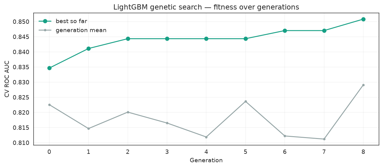

The num_leaves / max_depth interaction

Each evaluated candidate is plotted by its num_leaves and max_depth and colored by CV score. The productive region respects num_leaves ≤ 2^max_depth — the search concentrates there instead of wasting effort on invalid or overfitting combinations.

results = pd.DataFrame(ga_search.cv_results_)
fig, ax = plt.subplots(figsize=(8, 5))
sc = ax.scatter(results["param_max_depth"], results["param_num_leaves"],
                c=results["mean_test_score"], cmap="viridis", s=60, edgecolor="white")
depths = np.arange(3, 15)
ax.plot(depths, 2.0 ** depths, "--", color="crimson", label="num_leaves = 2^max_depth")
ax.set_ylim(0, 270)
ax.set_xlabel("max_depth")
ax.set_ylabel("num_leaves")
ax.set_title("Evaluated candidates, colored by CV ROC AUC")
ax.legend(frameon=False)
fig.colorbar(sc, label="mean CV ROC AUC")
fig.tight_layout()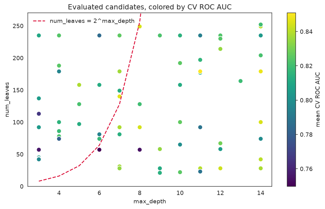

Practical Notes

• num_leaves is LightGBM's primary complexity knob — always tune it together with max_depth, never in isolation.
• Pair n_jobs=1 on the estimator with parallel_backend="cv" to avoid CPU oversubscription.
• The headline win is tuning vs the default model; the search finds a configuration that generalizes better on noisy data.
• verbose=-1 keeps LightGBM quiet so the generation log stays readable.

See Also

• Tune XGBoost — level-wise boosting and the same workflow
• Tune CatBoost — ordered boosting and CatBoost-specific knobs
• Advanced Optimizer Control