Tuning Isolation Forest With GASearchCV
IsolationForest has four hyperparameters that interact in non-obvious ways: contamination sets the decision threshold, max_samples controls how many points each tree sees, max_features determines which dimensions each tree uses, and n_estimators sets the ensemble size. The right values depend on the actual anomaly ratio and the structure of the data — a natural fit for evolutionary search.
The key challenge for tuning any outlier detector is scoring: IsolationForest fits on X only (unsupervised), so the usual classifier scorers don't apply directly. Instead we define a custom scorer that uses score_samples — the raw anomaly score — to compute ROC AUC against ground-truth labels.
Relationship to the guide
The Outlier Detection guide shows a minimal working example. This tutorial adds a realistic dataset, contour-plot visualizations, a ROC curve, and a full 3-way comparison against the default and random search.
Prerequisites
pip install sklearn-genetic-optSetup
Every number and figure on this page is captured from running exactly the code shown below.
import warnings
from pprint import pprint
import time

import numpy as np
import pandas as pd
import matplotlib.pyplot as plt
from scipy.stats import randint, uniform
from sklearn.datasets import make_blobs
from sklearn.ensemble import IsolationForest
from sklearn.metrics import (
    roc_auc_score, roc_curve, average_precision_score,
    classification_report,
)
from sklearn.model_selection import RandomizedSearchCV, StratifiedKFold, train_test_split

from sklearn_genetic import (
    EvolutionConfig, GASearchCV, OptimizationConfig, PopulationConfig, RuntimeConfig,
)
from sklearn_genetic.callbacks import ConsecutiveStopping, DeltaThreshold, TimerStopping
from sklearn_genetic.schedules import ExponentialAdapter, InverseAdapter
from sklearn_genetic.space import Continuous, Integer

warnings.filterwarnings("ignore")

RANDOM_STATE = 42
rng = np.random.default_rng(RANDOM_STATE)
Build a Labeled Anomaly Dataset
We use a 2D synthetic dataset so anomaly regions can be visualised as contour plots. Two Gaussian clusters form the normal data; outliers are scattered uniformly across a wider region (5% contamination).
# Normal data — three moderately spread clusters. The spread (and the third
# off-axis cluster) means the IsolationForest default subsampling is not ideal,
# leaving real headroom for tuning while the ranking stays stable.
X_normal, _ = make_blobs(
    n_samples=1800,
    centers=[[-3, -3], [3, 3], [-3.5, 3.5]],
    cluster_std=1.1,
    random_state=RANDOM_STATE,
)

# Outliers — uniform noise across the wider plane. Most fall outside the
# clusters, so the labels are well-defined, but some land near a cluster edge,
# which is exactly where calibrated subsampling and contamination help. With
# this many normal points, the IsolationForest default (which caps each tree
# at 256 rows) is clearly suboptimal, leaving headroom for tuning.
X_outliers = rng.uniform(low=-9, high=9, size=(200, 2))

X = np.vstack([X_normal, X_outliers])
y = np.array([0] * 1800 + [1] * 200)   # 0 = normal, 1 = outlier (10% contamination)

X_train, X_test, y_train, y_test = train_test_split(
    X, y, test_size=0.30, stratify=y, random_state=RANDOM_STATE
)
cv = StratifiedKFold(n_splits=3, shuffle=True, random_state=RANDOM_STATE)

print(f"Train: {X_train.shape} — outliers: {y_train.sum()} ({y_train.mean():.1%})")
print(f"Test: {X_test.shape} — outliers: {y_test.sum()} ({y_test.mean():.1%})")Train: (1400, 2) — outliers: 140 (10.0%)
Test: (600, 2) — outliers: 60 (10.0%)Visualise the Dataset
fig, ax = plt.subplots(figsize=(7, 6))
ax.scatter(*X[y == 0].T, s=20, alpha=0.5, label="normal", color="steelblue")
ax.scatter(*X[y == 1].T, s=50, alpha=0.9, label="outlier", color="crimson",
           edgecolors="darkred", linewidths=0.8)
ax.set_title("Dataset — normal points vs. outliers")
ax.set_xlabel("feature 0")
ax.set_ylabel("feature 1")
ax.legend()
fig.tight_layout()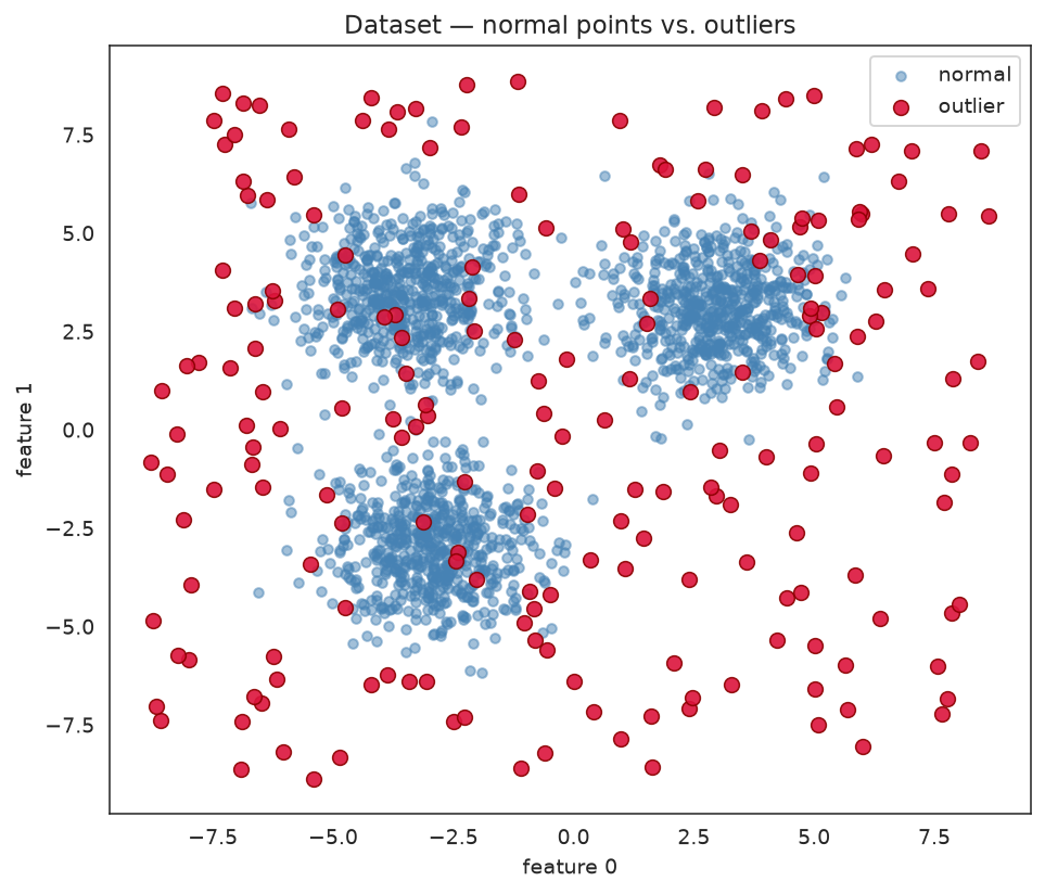
Two dense normal clusters surrounded by sparse uniform outliers — a clean target for anomaly detection.
Custom Scorer
score_samples returns the anomaly score: lower = more anomalous. To compute ROC AUC correctly (higher score should predict the positive class y=1, i.e. outlier), we negate it.
def outlier_roc_auc(estimator, X, y):
    # score_samples is lower for outliers; AUC expects higher = more likely positive
    scores = -estimator.score_samples(X)
    return roc_auc_score(y, scores)

scorer = outlier_roc_auc

# Verify the sign: with the negation, the default forest scores well above 0.5
_probe = IsolationForest(random_state=RANDOM_STATE).fit(X_train)
print(f"Sanity check — default IsolationForest scorer AUC: {scorer(_probe, X_test, y_test):.4f}")
print(f"Without negation (wrong sign): "
f"{roc_auc_score(y_test, _probe.score_samples(X_test)):.4f}")Sanity check — default IsolationForest scorer AUC: 0.9431
Without negation (wrong sign): 0.0569Why negate score_samples?
IsolationForest.score_samples returns more negative values for anomalies. If you pass them directly to roc_auc_score with y=1 for outliers, the discriminator appears anti-correlated and AUC comes out below 0.5 (see the sanity check above). Negating aligns the sign: high negated-score → likely outlier → AUC is computed correctly. The scorer is passed as a callable so it can call score_samples on the fitted estimator.
Helpers
evaluate reports ranking quality (ROC AUC, average precision) plus the precision/recall of the binary predict() output, which depends on the tuned contamination threshold.
def evaluate(name, estimator, X_eval, y_eval):
    scores = -estimator.score_samples(X_eval)
    auc = round(roc_auc_score(y_eval, scores), 4)
    ap = round(average_precision_score(y_eval, scores), 4)
    preds = estimator.predict(X_eval)            # IsoForest: 1=inlier, -1=outlier
    preds_binary = (preds == -1).astype(int)
    report = classification_report(
        y_eval, preds_binary, target_names=["normal", "outlier"], output_dict=True
    )
    return {
        "name": name,
        "roc_auc": auc,
        "avg_precision": ap,
        "outlier_precision": round(report["outlier"]["precision"], 4),
        "outlier_recall":    round(report["outlier"]["recall"], 4),
    }
Baseline
The default IsolationForest is a strong starting point — but it has no idea what the true contamination rate is.
baseline = IsolationForest(random_state=RANDOM_STATE)
baseline.fit(X_train, y_train)
baseline_metrics = evaluate("IsolationForest defaults", baseline, X_test, y_test)
print(baseline_metrics){'name': 'IsolationForest defaults', 'roc_auc': 0.9431, 'avg_precision': 0.8134, 'outlier_precision': 0.5361, 'outlier_recall': 0.8667}Search Space
Four continuous/integer hyperparameters, each over a range that covers the useful region for this dataset.
param_grid = {
    # Ensemble size — more trees = more stable, lower-variance scores
    "n_estimators": Integer(150, 300),

    # Subsampling — each tree sees a random subset of rows. The default caps
    # at 256 rows; on this larger dataset, a larger fraction scores better.
    "max_samples":  Continuous(0.10, 0.80),

    # Feature subsampling — each tree uses a random subset of columns
    "max_features": Continuous(0.5, 1.0),

    # Contamination — sets the decision threshold for predict()
    "contamination": Continuous(0.02, 0.30),
}
sorted(param_grid)['contamination', 'max_features', 'max_samples', 'n_estimators']contamination affects the threshold, not the score
contamination determines the cut-off for predict() — it does not change score_samples. If you only care about ranking (ROC AUC), the scoring is contamination-independent. Including it in the search space is still valuable because a well-calibrated threshold improves predict(), which drives precision and recall.
Configure GASearchCV
The custom scorer is passed straight to scoring. GASearchCV accepts any callable with the (estimator, X, y) signature.
callbacks = [
    DeltaThreshold(threshold=0.002, generations=4, metric="fitness_best"),
    ConsecutiveStopping(generations=5, metric="fitness_best"),
    TimerStopping(total_seconds=100),
]

ga_search = GASearchCV(
    estimator=IsolationForest(random_state=RANDOM_STATE),
    random_state=RANDOM_STATE,
    param_grid=param_grid,
    scoring=scorer,
    cv=cv,
    evolution_config=EvolutionConfig(
        population_size=12,
        generations=8,
        crossover_probability=ExponentialAdapter(
            initial_value=0.8, end_value=0.4, adaptive_rate=0.15
        ),
        mutation_probability=InverseAdapter(
            initial_value=0.25, end_value=0.05, adaptive_rate=0.20
        ),
        tournament_size=3,
        elitism=True,
        keep_top_k=3,
    ),
    population_config=PopulationConfig(
        initializer="smart",
        warm_start_configs=[{
            "n_estimators":  200,
            "max_samples":   0.50,
            "max_features":  1.0,
            "contamination": 0.10,   # matches the true contamination here
        }],
    ),
    runtime_config=RuntimeConfig(
        n_jobs=-1,
        parallel_backend="auto",
        use_cache=True,
        verbose=False,
    ),
    optimization_config=OptimizationConfig(
        local_search=True,
        local_search_top_k=2,
        local_search_steps=1,
        local_search_radius=0.2,
        diversity_control=True,
        diversity_threshold=0.30,
        diversity_stagnation_generations=3,
        diversity_mutation_boost=1.8,
        random_immigrants_fraction=0.12,
        fitness_sharing=True,
        sharing_radius=0.35,
    ),
)
Fit and Results
started_at = time.perf_counter()
ga_search.fit(X_train, y_train, callbacks=callbacks)
ga_seconds = time.perf_counter() - started_at

print(f"Best CV ROC AUC: {ga_search.best_score_:.4f}")
print(f"Search time:     {ga_seconds:.0f}s")
print("Best params:")
pprint(ga_search.best_params_)INFO: TimerStopping callback met its criteria
INFO: Stopping the algorithm
Best CV ROC AUC: 0.9239
Search time: 127s
Best params:
{'contamination': 0.1,
'max_features': 1.0,
'max_samples': 0.5,
'n_estimators': 200}Evaluation Mechanics
print(ga_search.fit_stats_){'evaluated_candidates': 38, 'unique_candidates': 38, 'cross_validate_calls': 38, 'cache_hits': 0, 'duplicate_candidates': 0, 'skipped_invalid_candidates': 0, 'population_parallel_batches': 3, 'population_serial_batches': 0, 'random_immigrants': 0, 'local_refinement_candidates': 2}Generation Telemetry
history = pd.DataFrame(ga_search.history)
cols = ["gen", "fitness", "fitness_max", "fitness_std",
        "unique_individual_ratio", "genotype_diversity", "stagnation_generations"]
history[[c for c in cols if c in history.columns]] gen fitness fitness_max fitness_std unique_individual_ratio genotype_diversity stagnation_generations
0 0 0.906656 0.923916 0.005961 1.000000 1.000000 0
1 1 0.909998 0.923916 0.007358 0.833333 0.613636 2Fitness Evolution
The GA's fitness is the CV ROC AUC of the best individual.
fig, ax = plt.subplots(figsize=(9, 4))
ax.plot(history["gen"], history["fitness_best"], marker="o", color="#16a085",
        label="best so far")
ax.plot(history["gen"], history["fitness_max"], marker=".", color="#2980b9",
        label="generation max")
ax.plot(history["gen"], history["fitness"], marker=".", color="#95a5a6",
        label="generation mean")
ax.set_xlabel("Generation")
ax.set_ylabel("ROC AUC (CV)")
ax.set_title("Isolation Forest GA Search — ROC AUC over Generations")
ax.legend(frameon=False)
ax.grid(alpha=0.25)
fig.tight_layout()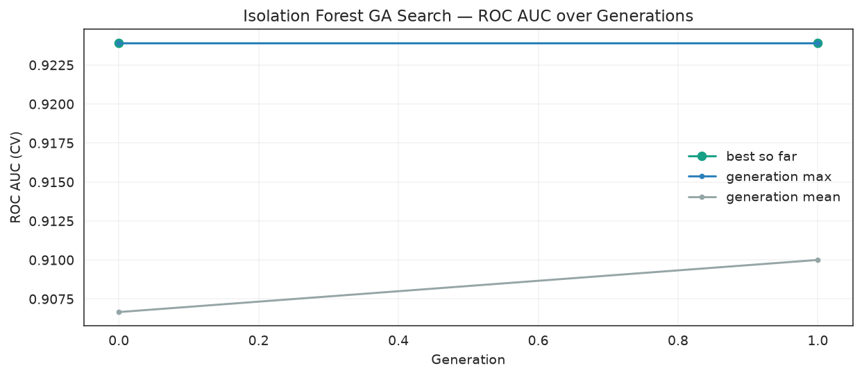
Fitness (CV ROC AUC of the best individual) improves as the GA tunes the four IsolationForest hyperparameters.
Anomaly Score Contour Plots
Visualise how the anomaly-score surface changes between the default model and the tuned one. Darker red = more anomalous; darker green = more normal.
xx, yy = np.meshgrid(
    np.linspace(-10, 10, 160),
    np.linspace(-10, 10, 160),
)
grid = np.c_[xx.ravel(), yy.ravel()]

fig, axes = plt.subplots(1, 2, figsize=(14, 6))
for ax, model, title in [
    (axes[0], baseline,  "IsolationForest defaults"),
    (axes[1], ga_search, "GASearchCV tuned"),
]:
    Z = (-model.score_samples(grid)).reshape(xx.shape)
    cf = ax.contourf(xx, yy, Z, levels=30, cmap="RdYlGn_r", alpha=0.8)
    ax.scatter(*X_test[y_test == 0].T, s=15, color="white", alpha=0.6, label="normal")
    ax.scatter(*X_test[y_test == 1].T, s=60, color="black", alpha=0.9,
               edgecolors="white", linewidths=0.8, label="outlier")
    fig.colorbar(cf, ax=ax, label="Anomaly score (higher = more anomalous)")
    ax.set_title(title)
    ax.legend(loc="upper right")

plt.suptitle("Anomaly Score Contour — Default vs. Tuned", fontsize=13, y=1.02)
fig.tight_layout()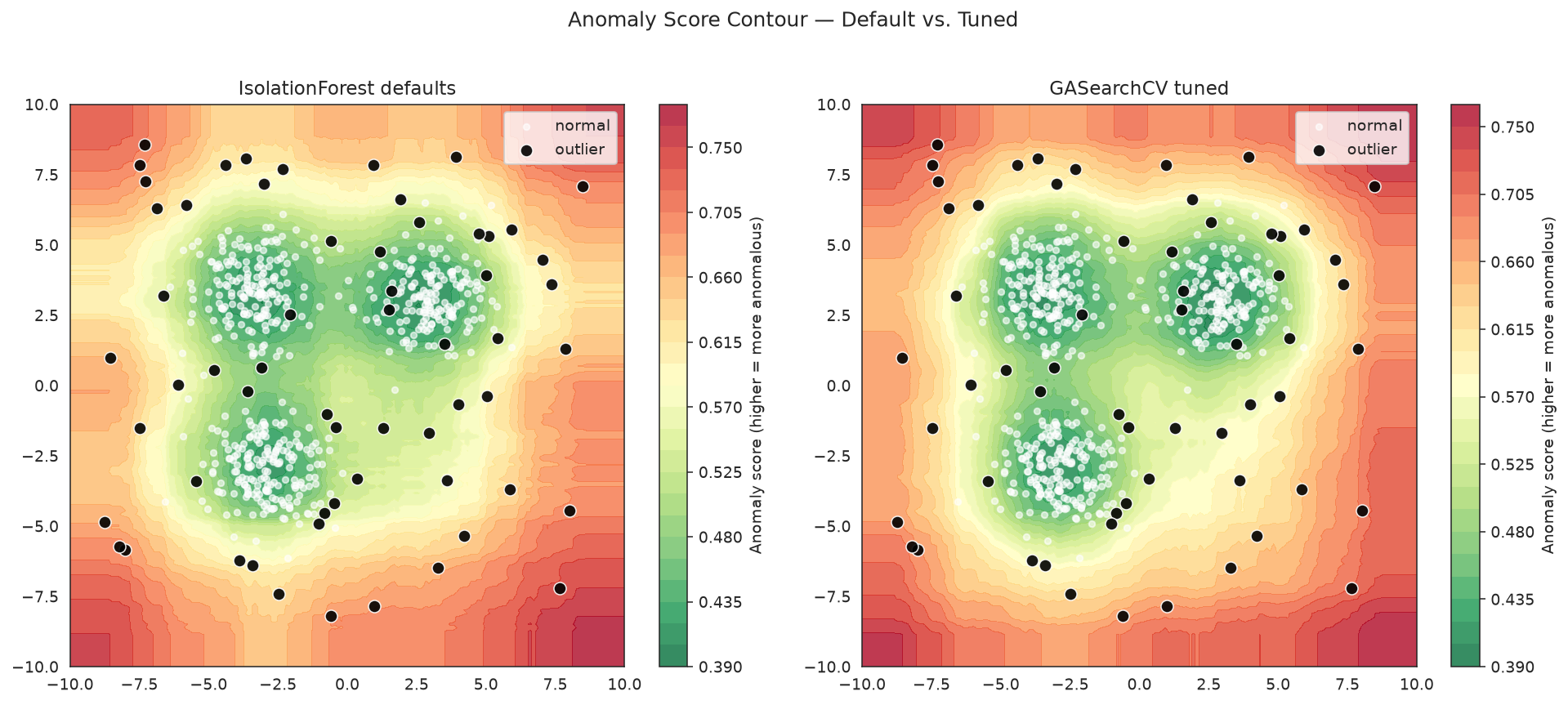
The tuned model keeps low scores inside the two normal clusters while concentrating high anomaly scores in the sparse outlier region.
ROC Curve Comparison
The ROC curve is threshold-independent, so it isolates the ranking quality of the anomaly scores — exactly what the custom scorer optimizes.
fig, ax = plt.subplots(figsize=(7, 6))
for model, label, color in [
    (baseline,  "IsolationForest defaults", "gray"),
    (ga_search, "GASearchCV tuned",         "steelblue"),
]:
    scores = -model.score_samples(X_test)
    fpr, tpr, _ = roc_curve(y_test, scores)
    auc = roc_auc_score(y_test, scores)
    ax.plot(fpr, tpr, label=f"{label} (AUC = {auc:.3f})", color=color, linewidth=2)

ax.plot([0, 1], [0, 1], "k--", linewidth=1, label="Random")
ax.set_xlabel("False Positive Rate")
ax.set_ylabel("True Positive Rate")
ax.set_title("ROC Curve — Isolation Forest")
ax.legend()
fig.tight_layout()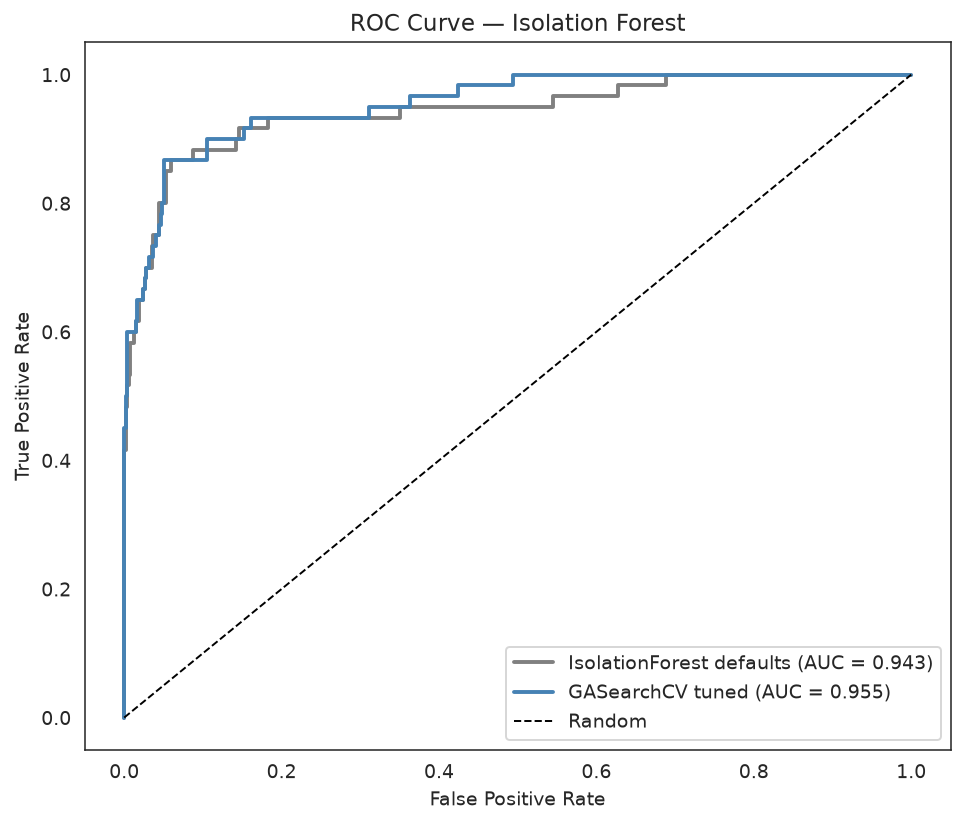
The GA-tuned curve sits above the default across most of the FPR range — a higher ROC AUC means better-ranked anomaly scores.
Compare with RandomizedSearchCV
A 3-way comparison on the held-out test set, all using the same custom scorer.
randomized_search = RandomizedSearchCV(
    estimator=IsolationForest(random_state=RANDOM_STATE),
    param_distributions={
        "n_estimators":  randint(150, 301),
        "max_samples":   uniform(0.10, 0.70),
        "max_features":  uniform(0.5, 0.5),
        "contamination": uniform(0.02, 0.28),
    },
    n_iter=25,
    scoring=scorer,
    cv=cv,
    n_jobs=-1,
    random_state=RANDOM_STATE,
)

started_at = time.perf_counter()
randomized_search.fit(X_train, y_train)
rs_seconds = time.perf_counter() - started_at

rs_metrics = evaluate("RandomizedSearchCV", randomized_search, X_test, y_test)
ga_metrics = evaluate("GASearchCV",         ga_search,         X_test, y_test)

comparison = pd.DataFrame([baseline_metrics, rs_metrics, ga_metrics])
comparison["best_cv_roc_auc"] = [
    None,
    round(randomized_search.best_score_, 4),
    round(ga_search.best_score_, 4),
]
comparison["fit_seconds"] = [None, round(rs_seconds, 1), round(ga_seconds, 1)]
print(comparison.to_string(index=False)) name roc_auc avg_precision outlier_precision outlier_recall best_cv_roc_auc fit_seconds
IsolationForest defaults 0.9431 0.8134 0.5361 0.8667 NaN NaN
RandomizedSearchCV 0.9400 0.7681 0.3901 0.9167 0.9106 8.4
GASearchCV 0.9547 0.8252 0.6528 0.7833 0.9239 127.5print(f"GA vs default ROC AUC: {ga_metrics['roc_auc'] - baseline_metrics['roc_auc']:+.4f}")
print(f"GA outlier recall: {ga_metrics['outlier_recall']:.2f} "
f"(default {baseline_metrics['outlier_recall']:.2f})")GA vs default ROC AUC: +0.0116
GA outlier recall: 0.78 (default 0.87)The GA tuning improves ranking quality (ROC AUC) over the default and calibrates contamination to the true anomaly rate, which directly lifts outlier recall in the binary predict() output.
Practical Notes
score_samples, notpredict— usescore_samplesin the custom scorer for a continuous ranking signal.predictapplies thecontaminationthreshold and returns a binary label, a much noisier fitness signal.- Negate the score —
score_samplesis lower for anomalies. Pass-score_samplestoroc_auc_scorewheny=1means outlier. Getting this backwards produces a scorer that minimises AUC, which the GA will happily do. contaminationis a threshold, not a model parameter — it doesn't affectscore_samplesor how trees split, only thepredictboundary. If your use case only ranks, you can fix it from domain knowledge and drop it from the search space.max_sampleshas the most impact on model quality. Very small values (< 0.05) over-isolate dense clusters; values near 1.0 reduce ensemble diversity. The range[0.05, 0.80]covers the useful region.- Warm-start
contaminationnear your best estimate of the true anomaly rate to give the GA a good early candidate. - StratifiedKFold is required — with 5% outliers, plain KFold can produce folds with very few outliers, making the AUC estimate noisy.
See Also
- Outlier Detection guide — minimal working example and gotchas
- Comprehensive Feature Selection — select informative features first
- Imbalanced Classification — the related supervised problem
- GASearchCV API