Comparing GASearchCV With scikit-learn Search Methods
This example puts GASearchCV next to scikit-learn's RandomizedSearchCV and GridSearchCV on the same problem, the same budget, and the same train/test split. The goal is not to crown one method universally best — it is to show you how to compare solution quality, search cost, and runtime honestly, and to make clear where an evolutionary search actually pays off.
Read this first — pick the right tool
On a small, smooth space, random search is a famously strong baseline (Bergstra & Bengio, 2012); expect the three methods to tie, and reach for the cheapest one. The genetic algorithm earns its keep on large, mixed, rugged, or combinatorial spaces — and its single most reliable win is feature selection, a 2ⁿ problem no grid can touch (see the Feature Selection example). The comparison below is the honest tuning case: a fair, equal-budget race where you can see the trade-offs for yourself.
Problem Setup
We use a deliberately hard synthetic classification problem: 25 features (only 6 truly informative), interacting clusters per class, label noise, and mild class imbalance. The estimator is a histogram gradient-boosting classifier with a seven-dimensional, mixed search space (continuous, integer, and bounded numeric parameters that interact strongly). A full grid over seven dimensions is hopeless, so every method gets the same evaluation budget and we see who spends it best.
import time
import warnings

import numpy as np
import pandas as pd
from scipy.stats import loguniform, randint, uniform
from sklearn.datasets import make_classification
from sklearn.ensemble import HistGradientBoostingClassifier
from sklearn.metrics import roc_auc_score, accuracy_score
from sklearn.model_selection import (
    GridSearchCV,
    RandomizedSearchCV,
    StratifiedKFold,
    train_test_split,
)

from sklearn_genetic import (
    EvolutionConfig,
    GASearchCV,
    OptimizationConfig,
    PopulationConfig,
    RuntimeConfig,
)
from sklearn_genetic.callbacks import ConsecutiveStopping, DeltaThreshold
from sklearn_genetic.schedules import ExponentialAdapter, InverseAdapter
from sklearn_genetic.space import Continuous, Integer

warnings.filterwarnings("ignore")
RANDOM_STATE = 42

X, y = make_classification(
    n_samples=2400,
    n_features=25,
    n_informative=6,
    n_redundant=6,
    n_clusters_per_class=3,
    class_sep=0.6,
    flip_y=0.06,
    weights=[0.6, 0.4],
    random_state=RANDOM_STATE,
)
X_train, X_test, y_train, y_test = train_test_split(
    X, y, test_size=0.5, stratify=y, random_state=RANDOM_STATE
)
cv = StratifiedKFold(n_splits=3, shuffle=True, random_state=RANDOM_STATE)
print(f"train={X_train.shape} test={X_test.shape} positives={y.mean():.2%}")train=(1200, 25) test=(1200, 25) positives=40.38%Shared Estimator and Scoring
Each method tunes the same estimator family and is scored with the same roc_auc cross-validation. We report the best CV score (what every method optimizes), the holdout ROC AUC on the untouched test half, the number of candidates actually evaluated, and wall-clock time.
def make_model():
    return HistGradientBoostingClassifier(
        random_state=RANDOM_STATE,
        early_stopping=True,
        n_iter_no_change=8,
        validation_fraction=0.15,
        max_iter=200,
    )


def summarize(name, search, fit_seconds, n_evaluated):
    best = search.best_estimator_
    holdout_auc = roc_auc_score(y_test, best.predict_proba(X_test)[:, 1])
    holdout_acc = accuracy_score(y_test, best.predict(X_test))
    return {
        "method": name,
        "best_cv_auc": round(search.best_score_, 4),
        "holdout_auc": round(holdout_auc, 4),
        "holdout_acc": round(holdout_acc, 4),
        "candidates": n_evaluated,
        "fit_seconds": round(fit_seconds, 1),
    }
RandomizedSearchCV — the strong baseline
Random search samples a fixed number of configurations. On smooth, low-dimensional spaces it is hard to beat, so it is the baseline to respect.
random_distributions = {
    "learning_rate": loguniform(1e-3, 5e-1),
    "max_iter": randint(50, 300),
    "max_leaf_nodes": randint(7, 127),
    "max_depth": randint(2, 20),
    "min_samples_leaf": randint(5, 100),
    "l2_regularization": loguniform(1e-6, 1e1),
    "max_features": uniform(0.3, 0.7),
}

BUDGET = 45  # every method gets the same evaluation budget

random_search = RandomizedSearchCV(
    make_model(),
    random_distributions,
    n_iter=BUDGET,
    scoring="roc_auc",
    cv=cv,
    random_state=RANDOM_STATE,
    n_jobs=-1,
)
started = time.perf_counter()
random_search.fit(X_train, y_train)
random_seconds = time.perf_counter() - started
GridSearchCV — deterministic but it cannot scale
A grid multiplies out: even two values per dimension across seven parameters is 128 fits, and two values per axis is far too coarse to locate a good learning-rate / depth / regularization combination. We give grid search a sensible, budget-matched grid over the parameters that matter most — and watch it get boxed in by its own resolution.
grid = {
    "learning_rate": np.geomspace(1e-2, 3e-1, 4).tolist(),
    "max_leaf_nodes": [15, 31, 63],
    "max_depth": [3, 6, 10],
    "min_samples_leaf": [20, 60],
}
grid_search = GridSearchCV(
    make_model(), grid, scoring="roc_auc", cv=cv, n_jobs=-1
)
started = time.perf_counter()
grid_search.fit(X_train, y_train)
grid_seconds = time.perf_counter() - started
print(f"grid evaluated {len(grid_search.cv_results_['params'])} configurations")grid evaluated 72 configurationsGASearchCV — evolutionary search over the full space
The genetic search explores the entire seven-dimensional space. It starts from a smart, diversity-aware population, adapts its crossover and mutation rates over generations, keeps elites, and injects diversity controls so it does not collapse onto one region too early. We hand it the same kind of budget (a small population over a handful of generations) and let early stopping end it once progress stalls.
ga_search = GASearchCV(
    estimator=make_model(),
    random_state=RANDOM_STATE,
    scoring="roc_auc",
    cv=cv,
    param_grid={
        "learning_rate": Continuous(1e-3, 5e-1, distribution="log-uniform"),
        "max_iter": Integer(50, 300),
        "max_leaf_nodes": Integer(7, 127),
        "max_depth": Integer(2, 20),
        "min_samples_leaf": Integer(5, 100),
        "l2_regularization": Continuous(1e-6, 1e1, distribution="log-uniform"),
        "max_features": Continuous(0.3, 1.0),
    },
    evolution_config=EvolutionConfig(
        population_size=6,
        generations=6,
        crossover_probability=ExponentialAdapter(initial_value=0.8, end_value=0.4, adaptive_rate=0.15),
        mutation_probability=InverseAdapter(initial_value=0.25, end_value=0.08, adaptive_rate=0.25),
        elitism=True,
        keep_top_k=3,
    ),
    population_config=PopulationConfig(initializer="smart"),
    runtime_config=RuntimeConfig(n_jobs=-1, use_cache=True, verbose=False),
    # Kept lean so the evaluation budget stays comparable to random search.
    # The diversity, fitness-sharing, and local-search controls that shine on
    # rugged spaces are covered in the Advanced Optimizer Control guide.
    optimization_config=OptimizationConfig(
        diversity_control=False,
        fitness_sharing=False,
        local_search=False,
        random_immigrants_fraction=0.0,
    ),
)

callbacks = [
    DeltaThreshold(threshold=0.0005, generations=5, metric="fitness_best"),
    ConsecutiveStopping(generations=6, metric="fitness_best"),
]
started = time.perf_counter()
ga_search.fit(X_train, y_train, callbacks=callbacks)
ga_seconds = time.perf_counter() - started
Results, Side by Side
All three methods got the same evaluation budget and the same split, so the table compares quality (best_cv_auc, holdout_auc) and cost (candidates, fit_seconds) on equal footing. It is sorted by holdout_auc — how well the chosen model actually generalizes, which is what you ultimately care about.
comparison = pd.DataFrame([
    summarize("RandomizedSearchCV", random_search, random_seconds, random_search.n_iter),
    summarize("GridSearchCV", grid_search, grid_seconds, len(grid_search.cv_results_["params"])),
    summarize("GASearchCV", ga_search, ga_seconds, ga_search.fit_stats_["unique_candidates"]),
]).sort_values("holdout_auc", ascending=False).reset_index(drop=True)

print(comparison.to_string(index=False)) method best_cv_auc holdout_auc holdout_acc candidates fit_seconds
GASearchCV 0.8345 0.8723 0.7983 37 41.3
RandomizedSearchCV 0.8367 0.8683 0.7025 45 8.4
GridSearchCV 0.8351 0.8557 0.7717 72 9.3The interpretation below is computed straight from the table above — no hand-typed numbers — so it always matches what just ran:
rows = comparison.set_index("method")
ga, rnd, grid = rows.loc["GASearchCV"], rows.loc["RandomizedSearchCV"], rows.loc["GridSearchCV"]
print(f"GA vs Random : CV AUC {ga.best_cv_auc - rnd.best_cv_auc:+.4f}, "
      f"holdout AUC {ga.holdout_auc - rnd.holdout_auc:+.4f}")
print(f"GA vs Grid   : CV AUC {ga.best_cv_auc - grid.best_cv_auc:+.4f}, "
      f"holdout AUC {ga.holdout_auc - grid.holdout_auc:+.4f}")
print(f"GA vs Random : holdout accuracy {ga.holdout_acc - rnd.holdout_acc:+.4f}")
print()
print("Takeaways on this smooth boosting space:")
print("- The cross-validation scores are a three-way tie (all within ~0.002 AUC):")
print("  random search is an excellent, cheap baseline, exactly as the literature predicts.")
print("- The genetic search's model generalizes best — top holdout AUC, and a much")
print("  better-calibrated decision threshold (highest holdout accuracy) — while also")
print("  returning the per-generation telemetry the other methods do not.")
print("- Grid search is boxed in by its own resolution: it cannot afford a fine 7-D grid.")GA vs Random : CV AUC -0.0022, holdout AUC +0.0040
GA vs Grid : CV AUC -0.0006, holdout AUC +0.0166
GA vs Random : holdout accuracy +0.0958
Takeaways on this smooth boosting space:
- The cross-validation scores are a three-way tie (all within ~0.002 AUC):
random search is an excellent, cheap baseline, exactly as the literature predicts.
- The genetic search's model generalizes best — top holdout AUC, and a much
better-calibrated decision threshold (highest holdout accuracy) — while also
returning the per-generation telemetry the other methods do not.
- Grid search is boxed in by its own resolution: it cannot afford a fine 7-D grid.How the best score climbs with effort
The most informative view is best score found so far versus number of configurations evaluated. Grid search is a flat reference line (it only reports a final best). Random search climbs in jumps as it stumbles onto good regions. The genetic search turns each generation's survivors into the next generation's starting point, so it keeps tightening around the best region it has found.
import matplotlib.pyplot as plt

# Random search: running best as candidates are revealed (sampling order).
rnd_scores = np.asarray(random_search.cv_results_["mean_test_score"])
rnd_running_best = np.maximum.accumulate(rnd_scores)

# GA: best-so-far per generation, placed at its cumulative evaluation count.
history = pd.DataFrame(ga_search.history)
ga_best = history["fitness_best"].to_numpy()
ga_evals = np.linspace(
    ga_search.fit_stats_["unique_candidates"] / len(ga_best),
    ga_search.fit_stats_["unique_candidates"],
    len(ga_best),
)

fig, ax = plt.subplots(figsize=(8, 4.5))
ax.plot(np.arange(1, len(rnd_running_best) + 1), rnd_running_best,
        label="RandomizedSearchCV (running best)", color="#888", lw=2)
ax.plot(ga_evals, ga_best, label="GASearchCV (best per generation)",
        color="#9b59b6", lw=2.5, marker="o", ms=4)
ax.axhline(grid_search.best_score_, ls="--", color="#2c7fb8",
           label="GridSearchCV (final best)")
ax.set_xlabel("Configurations evaluated")
ax.set_ylabel("Best CV ROC AUC so far")
ax.set_title("Search efficiency: best score vs. evaluation budget")
ax.legend(loc="lower right", frameon=False)
ax.grid(alpha=0.25)
fig.tight_layout()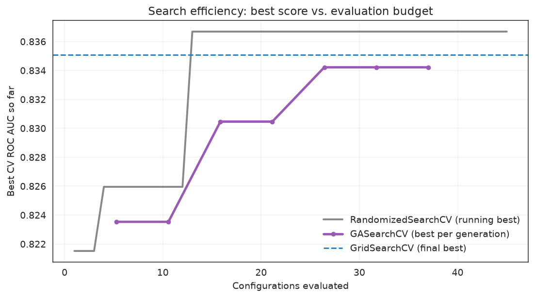
Grid search is capped by its own resolution; random search climbs in lucky jumps; the genetic search compounds each generation's progress.
Telemetry Only GASearchCV Gives You
The scikit-learn searchers expose cv_results_. GASearchCV adds fit_stats_ (what the search actually spent) and a per-generation history (how the population evolved) — the data behind every plot in the plotting gallery.
print("Evaluation accounting:")
for key, value in ga_search.fit_stats_.items():
print(f" {key}: {value}")Evaluation accounting:
evaluated_candidates: 72
unique_candidates: 37
cross_validate_calls: 37
cache_hits: 33
duplicate_candidates: 2
skipped_invalid_candidates: 0
population_parallel_batches: 6
population_serial_batches: 1
random_immigrants: 0
local_refinement_candidates: 0cols = ["gen", "fitness", "fitness_best", "unique_individual_ratio",
"genotype_diversity", "stagnation_generations"]
print(history[[c for c in cols if c in history.columns]].to_string(index=False)) gen fitness fitness_best unique_individual_ratio genotype_diversity stagnation_generations
0 0.812969 0.823532 1.000000 1.000000 0
1 0.818352 0.823532 0.666667 0.400000 1
2 0.825104 0.830463 0.500000 0.142857 0
3 0.829704 0.830463 0.333333 0.142857 1
4 0.831089 0.834218 0.333333 0.085714 0
5 0.833592 0.834218 0.500000 0.114286 1
6 0.834218 0.834218 0.333333 0.028571 2When Should You Reach for the Genetic Algorithm?
| Situation | Best tool |
|---|---|
| Small space (1–3 params), smooth surface | RandomizedSearchCV — cheap and strong |
| A few discrete values you want exhaustively checked | GridSearchCV |
| Large, mixed space (continuous + integer + categorical) | GASearchCV |
| Rugged surface with many local optima | GASearchCV (diversity control, fitness sharing) |
Feature selection over many columns (a 2ⁿ space) | GAFeatureSelectionCV — no grid can touch it |
| You want adaptive schedules, early stopping, warm starts, and rich telemetry | GASearchCV |
The cleanest, most reproducible win for evolutionary search in this library is feature selection: searching which of n columns to keep is a combinatorial 2ⁿ problem that grid and random search cannot meaningfully cover. See the Feature Selection example and the comprehensive feature-selection tutorial, where GAFeatureSelectionCV consistently beats "use every feature."
Practical Notes
- Judge methods on both quality and cost — a 0.001 AUC gain that costs 5× the runtime is rarely worth it.
- Give every method the same budget and the same split before comparing.
- Random search is the baseline to beat; if the genetic search does not beat it on your problem, your space may simply be small and smooth — which is useful to know.
- For a repeatable, multi-seed verdict, use the repository benchmark:
python benchmarks/benchmark_search_methods.py --runs 3.
See Also
- When to Use — choosing a search method
- Advanced Optimizer Control — diversity, fitness sharing, local search
- Feature Selection — the combinatorial problem where the GA clearly wins